The other day I encountered (and solved 😎 ) a creative problem while making interdependent drop downs in a dashboard. If one Item has been chosen in the first list then it should not appear in the second list and vice versa !!
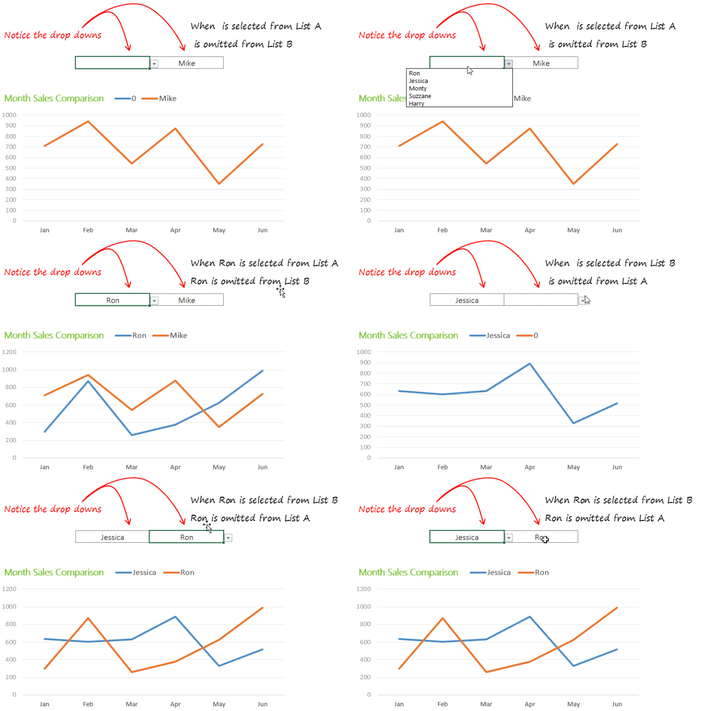
Check it out.. it is pretty cool !!
We start with a list of names
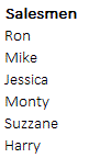 --> Let’s say we have six salesmen
Match the name in Drop down
I am using the MATCH function to find the row number of the selected item in the drop down. The reason of finding the row number is that I want to exclude the salesman selected in DrpDwnB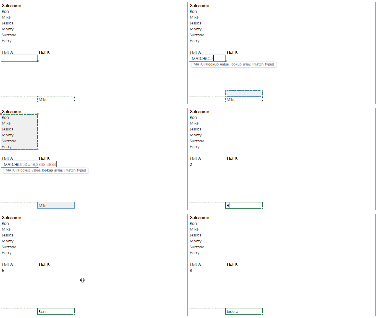
Please note a couple of things here
- I have named the drop down cell as DrpDwnB [learn cell naming here]
- I have also applied absolute cell referencing to the lookup array [learn cell referencing here]
Now give me all except this row number
Now that we have the row number of the salesmen and I want to exclude that row number from the list. So I am going to populate that with an IF based array formula. Array based formulas work with CTRL + SHIFT + ENTER
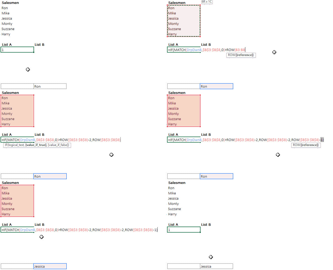
Digging into the formula
Don’t get scandalized, lets split the above formula into 3 parts and tame it down.. ready?
Part 1 MATCH – The match function (is continued) is extracting the row number, which is pretty straight forward

Part 2 IF TRUE – All records which are falling before the selected salesmen should give the same row number. Note that I have used ROW(list)-2 because our data is starting from the 3rd row and minus 2 will result in series of row numbers starting from 1

Part 3 IF FALSE – All records which are falling on or after the selected salesmen should give the next row number. That way we can skip the salesmen selected 😎

You can evaluate the formula by pressing F9 along the way. Now that is an array formula so we’ll press Ctrl + Shift + Enter after we finish writing it
Now pick up the nth smallest row number !
Now that we have the row numbers coming in, all we have to do is that our formula should pick up the 1st smallest row (when the formula is in the first row) moving to the largest row (when the formula is copied to the last row) that can be fixed with wrapping it around the SMALL function
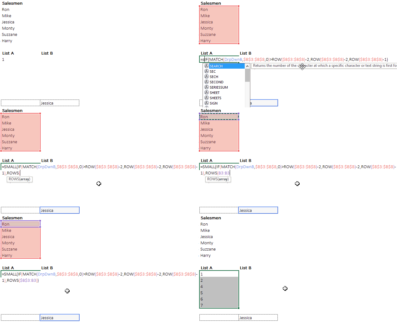
Note the expanding array (used in ROWS($B$3:B3) ) by freezing the first part of the range [learn how to make expanding arrays]
Finally populating the salesmen with the INDEX
We have the row numbers and our last stroke will be extracting the salesmen name but excluding the salesmen selected (which has been taken care of by the IF statement). Just wrap this monster around the INDEX and we are done!
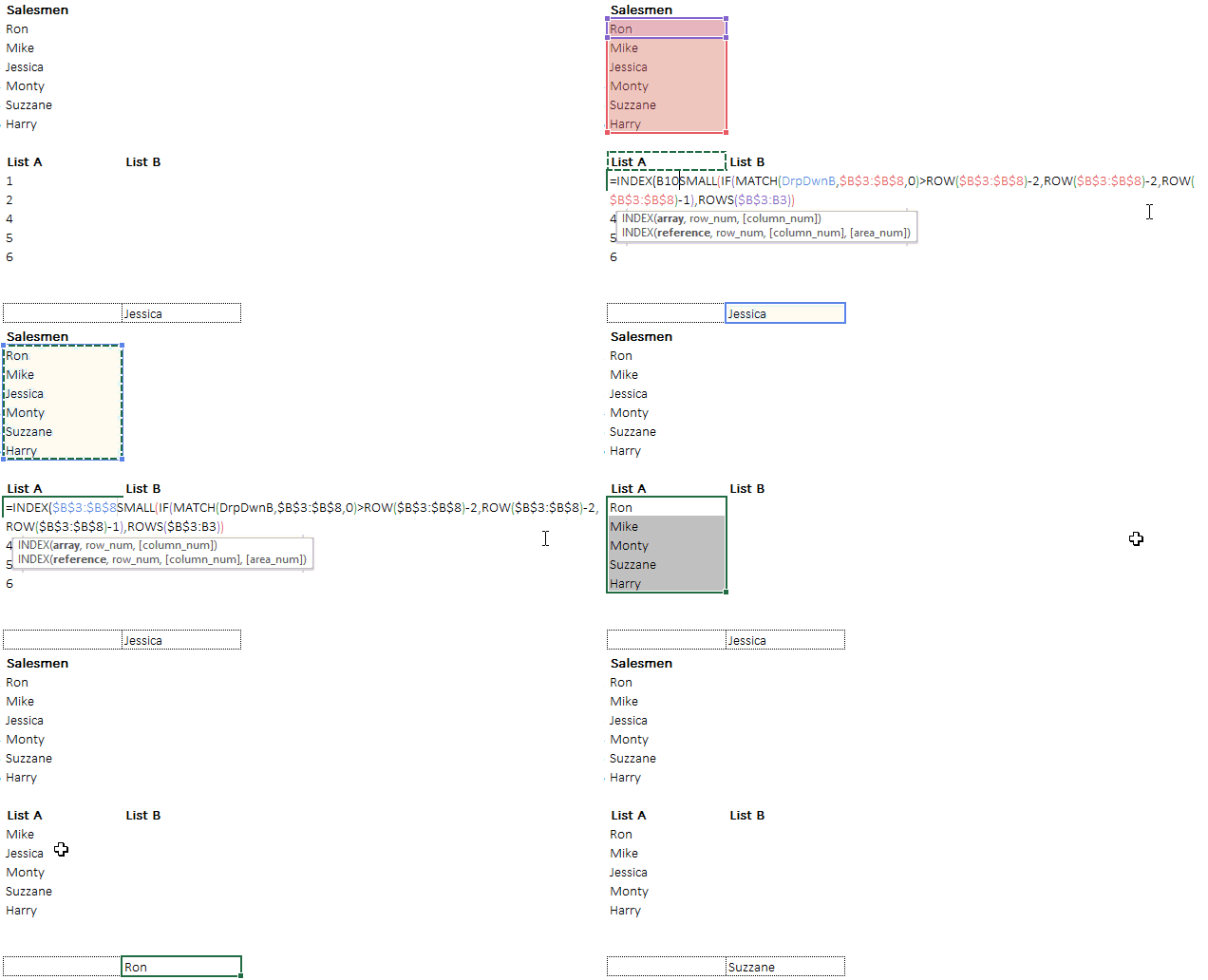
Notice that the any name typed in the drop down cell is not appearing in the list!!  Yeah I know it was lengthy but cool isn’t it?
Take look at one more example using INDEX and ROWS function
Similarly Create List B
All we have to do is copy the same formula and link the MATCH function to DrpdwnA.
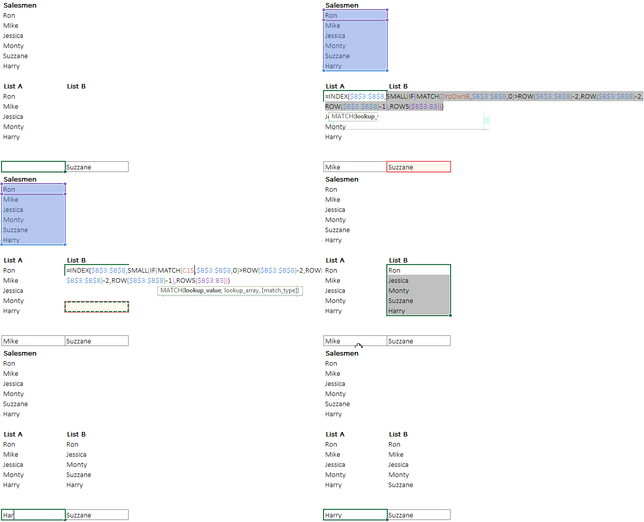
Creating Data Validation Dropdowns
Till now we have been typing names in the named drop down cells. Let’s name our 2 lists (A & B) and use data validation to create drop downs
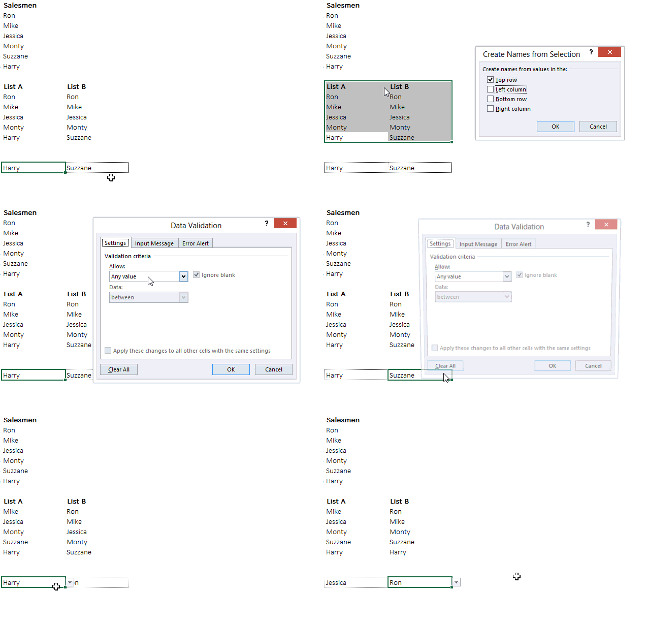
- Select both the lists and use the shortcut CTRL + SHIFT + F3 to open the naming dialogue box
- Since our names are kept in the top row, check only that option and press OK
- Now use Data Validation feature (shortcut ALT A V V) and link the named ranges as list drop downs
- No names that are in DrpdwnA will appear in Drpdwn B
Here is the file for you
Download the file from down below and play with it yourself!! Additionally I have added a chart using a simple Vlookup formula
When will this trick not work
I know I know.. it has been long that I have talking about this long formula alchemy but I am sure you don’t want to miss a small cautionary advice in the end. This formula will not work if the names (list items) repeat .. WHY because our dear MATCH function is just capable of picking the row number of only the first matched item from the list!!
Please do share your experiences with using this trick!