5 Quick Data Formatting Tips

Today let’s talk about some real quick and amazing formatting tricks to make your data look more presentable and I have 5 of them for you here! Enjoy 🙂

1. Dealing with Borders!

I have seen many people applying dark borders to their text, something like (shown below) The problem is that the jet black borders create distraction and the data becomes less readable

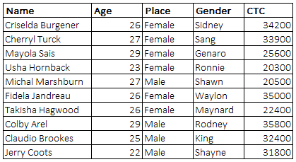
Try something like this instead. Simple borders will always make your data stand out. Remember the need for the border is just to separate the rows and even the light color does the job equally well

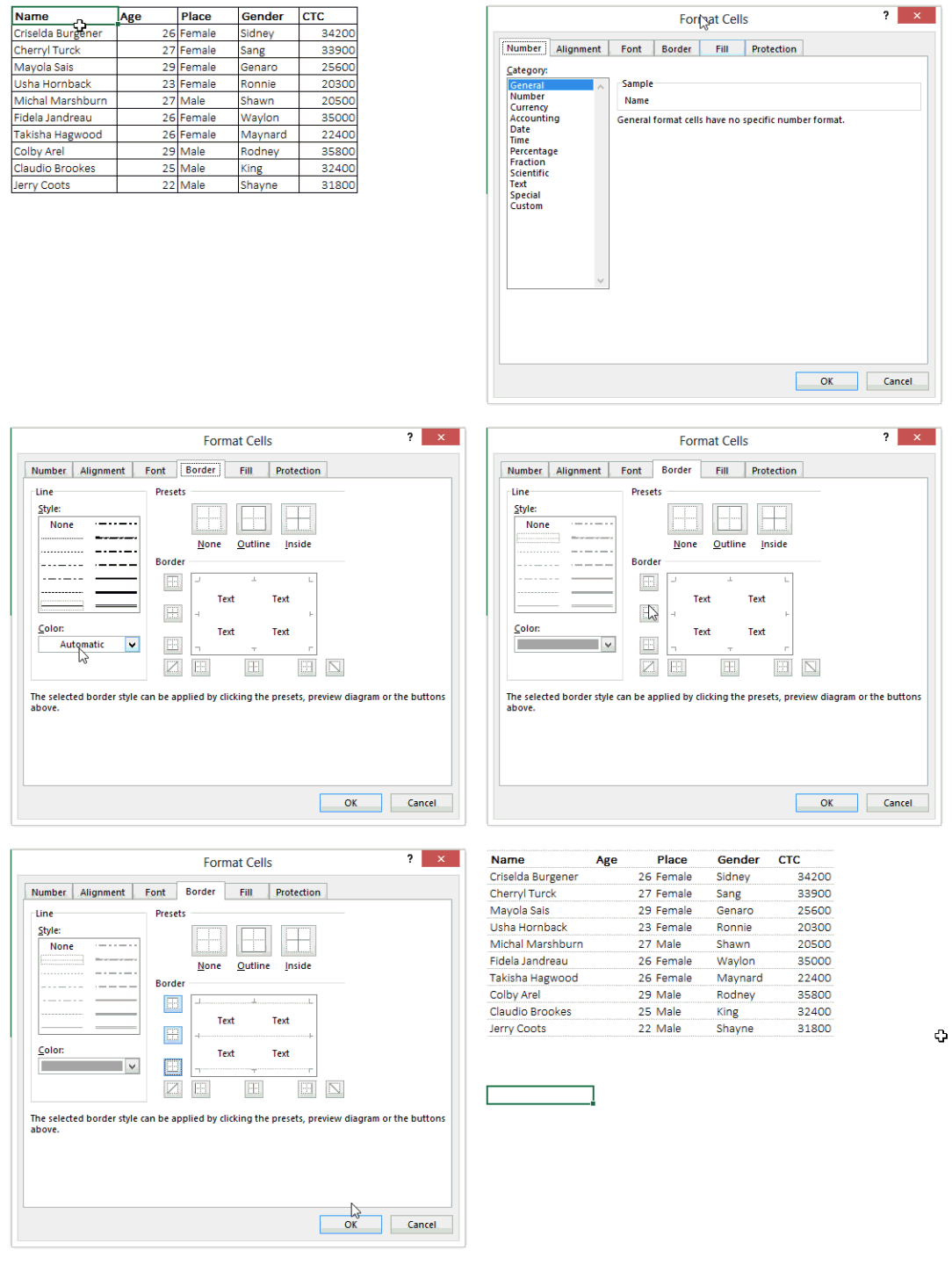
1. Select your data (with borders) and use Ctrl – minus sign to remove all borders
2. Now go to cell formatting dialogue box. You can find that option in the right click menu or use the shortcut Ctrl  1
3. In the Borders tab set the formatting options and apply light faded borders

Trust me it looks equally good on printouts as well

 

2. Use Paste Special in Charts

When I first got to know about this, it blew my mind off!! Let’s see how it works for you. You can use your old favorite  Paste Special in formatting charts really quick. I mean really quick!! Check it out!

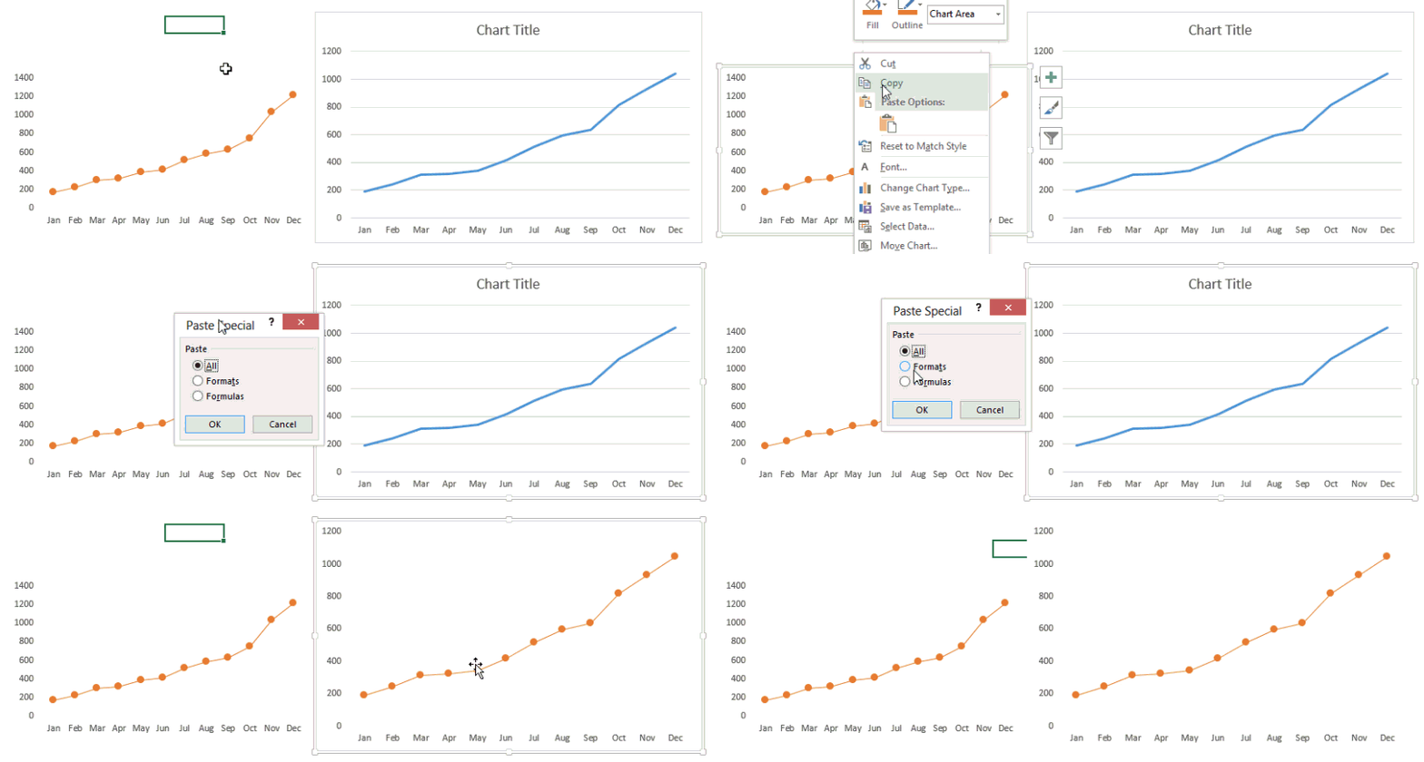
1. Copy the Chart from where you want to copy the formatting
2. Click on the unformatted chart and use Paste Special (ALT E S) option to paste the formats only
3. Ka..boom! done!

I find this insanely fast to copy the same formats to all my charts!

 

3. Clear all unwanted formatting at one shot!

Sometimes you just want to get rid of all unnecessary formatting done on the work sheet

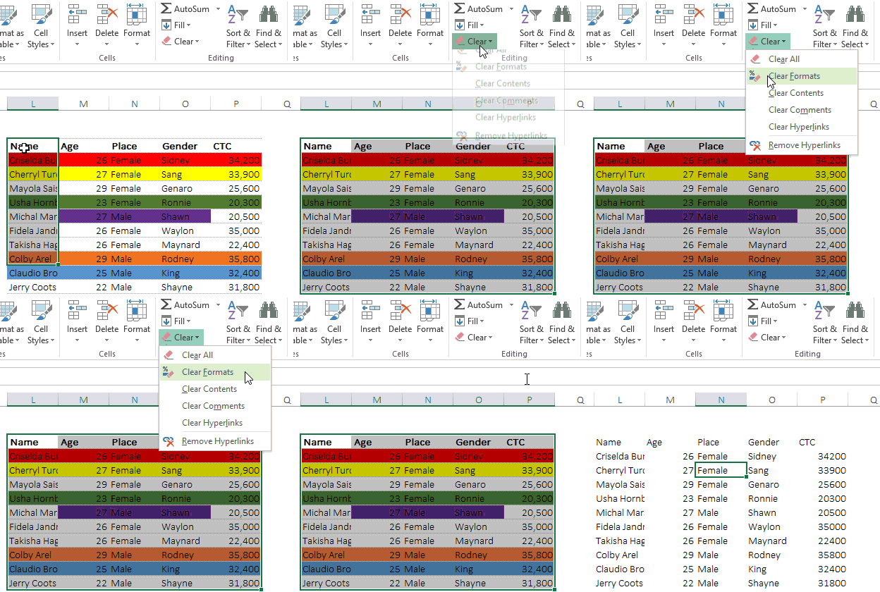
1. Use the simple shortcut ALT H E F
2. Or choose ‘Clear Format’ under the Clear option in the Home Tab

 

4. Grouping rows or Columns

When you have subset of any data you can group that into rows or columns. This solves two purpose

1. Grouping can hide rows and show up only if needed
2. Grouping creates a little icon on the rows numbering or column name panel that indicates that some data is grouped and can be pulled up by clicking at the button

 

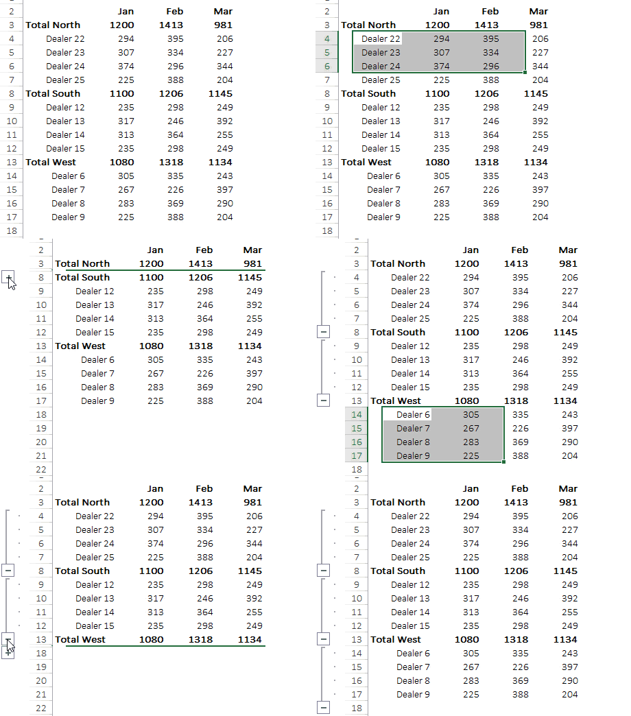
1. Select the data that you want to group
2. Go to Data Tab and choose the option Grouping and then click Rows to group rows
3. Alternatively you can also use the shortcut ALT A G G to access the grouping feature

Your data this way will look much better formatted!

 

5. Use Excel Tables

Excel Tables are by far the quickest way to format a set of data

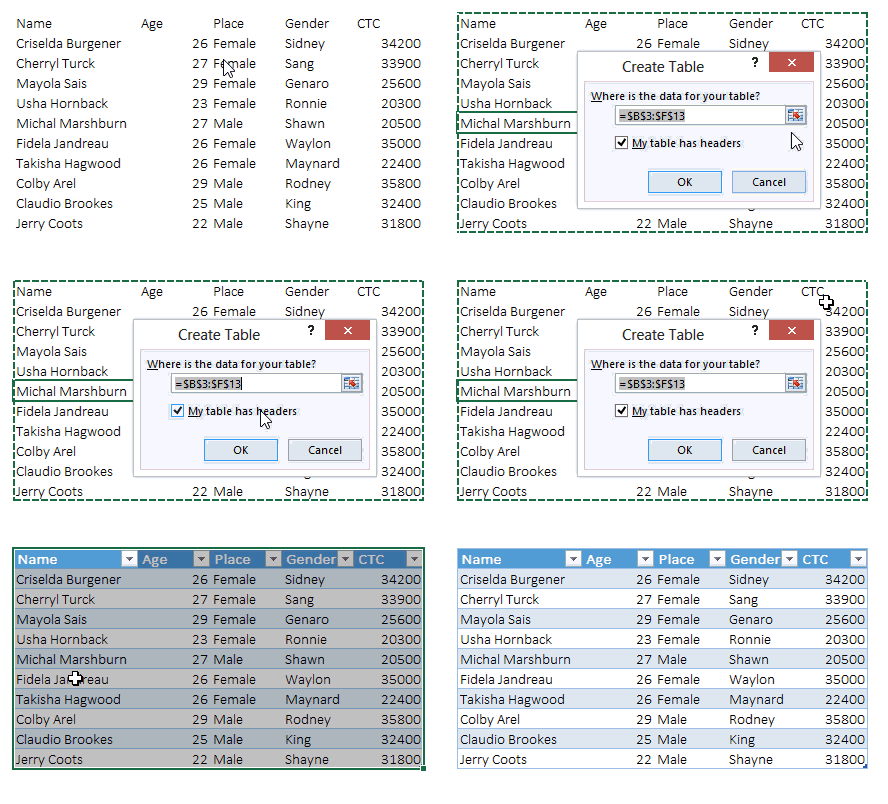
1. The active cell should be anywhere in the data range then press Ctrl T to activate Tables
2. A pop up will appear asking if your table has headers, preferably have headers in your data (that will benefit in writing formulas, we’ll cover that up later)
3. And your neatly formatted table is ready

Please note that Table is not a mere formatting feature, it is much more than that and insanely beneficial. I’ll write a short feature on Tables soon!!

 

Want some quick shortcuts on Excel & PowerPoint?

• Download Top 25 Excel key board shortcuts
• Download Top 12 PowerPoint shortcuts