Not so recently, one of our readers and a very avid questioner, Vidhat, asked me the following question

Let me explain with a little more detail!
Take a look at this data, we have ECode, Type and Amount
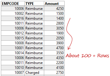
- An Employee Code can appear multiple times in this table
- The employee can ask for a reimbursement amount or the company can charge an amount from the employee
- The Problem – You want to calculate the net balance (+ve or -ve) i.e. Charged – Reimburse for each employee
How would you solve that using a Pivot Table?
Post your answers in the comments
Please post your interesting solutions in the comments and if you have a file to share, please paste a link to download the file.
I’ll also share 3 solutions (fragile to robust) that I found for this problem
Updated on 31st July 2017
Solution #1
Make a separate calculation outside of the Pivot Table. We do it all the time in case we want to calculate something that cannot be adjusted in the current pivot table calculation
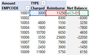
Just in case you get perturbed by GETPIVOTDATA Function that appears when you start writing the formula in the Pivot Table area, click here to turn off GETPIVOTDATA
This is one of the most lame and quick fix solutions that comes to mind in the first place. Let’s take a look at another one which slightly more robust
Solution 2
Use the Pivot Table built in Calculation method : Difference From
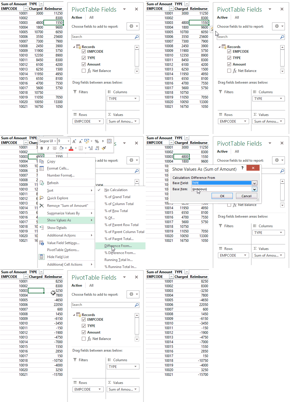
- Right Click on the Charged Column
- Go to Show Values as and select “Difference From”
- Base Field = “TYPE” and Base Item = “Charged”
- And you’ll get the difference between the two values
This method is cool but you’ll not be able to completely get rid of the extra empty column. Plus if you change the shape of the pivot table this calculation won’t work
Solution 3
Create a measure in PowerPivot and then add it to the pivot table. This method is by far the most robust method of all. Here is how it works
Step 1 : Add the data to the data model while creating a pivot table.
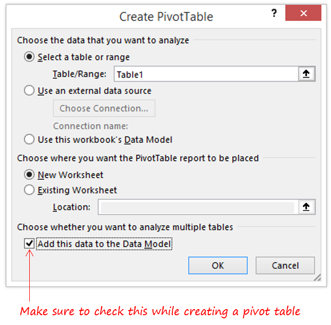
Note that : Data model feature is available starting Excel 2013 but you can manually load the data in PowerPivot window using Excel 2010 as well. Excel 2007 guys.. sorry you need an upgrade!
Step 2: Create a Measure

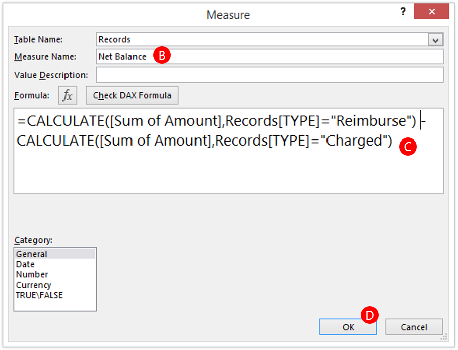
Once you have created a pivot table
- Right click on the Records Table in the pivot field list and choose “Add Measure”
- In the measure box – Give your measure a name
- Write the DAX Formula as shown
- OK
Step 3 : Add the measure “Net Balance” to the pivot table
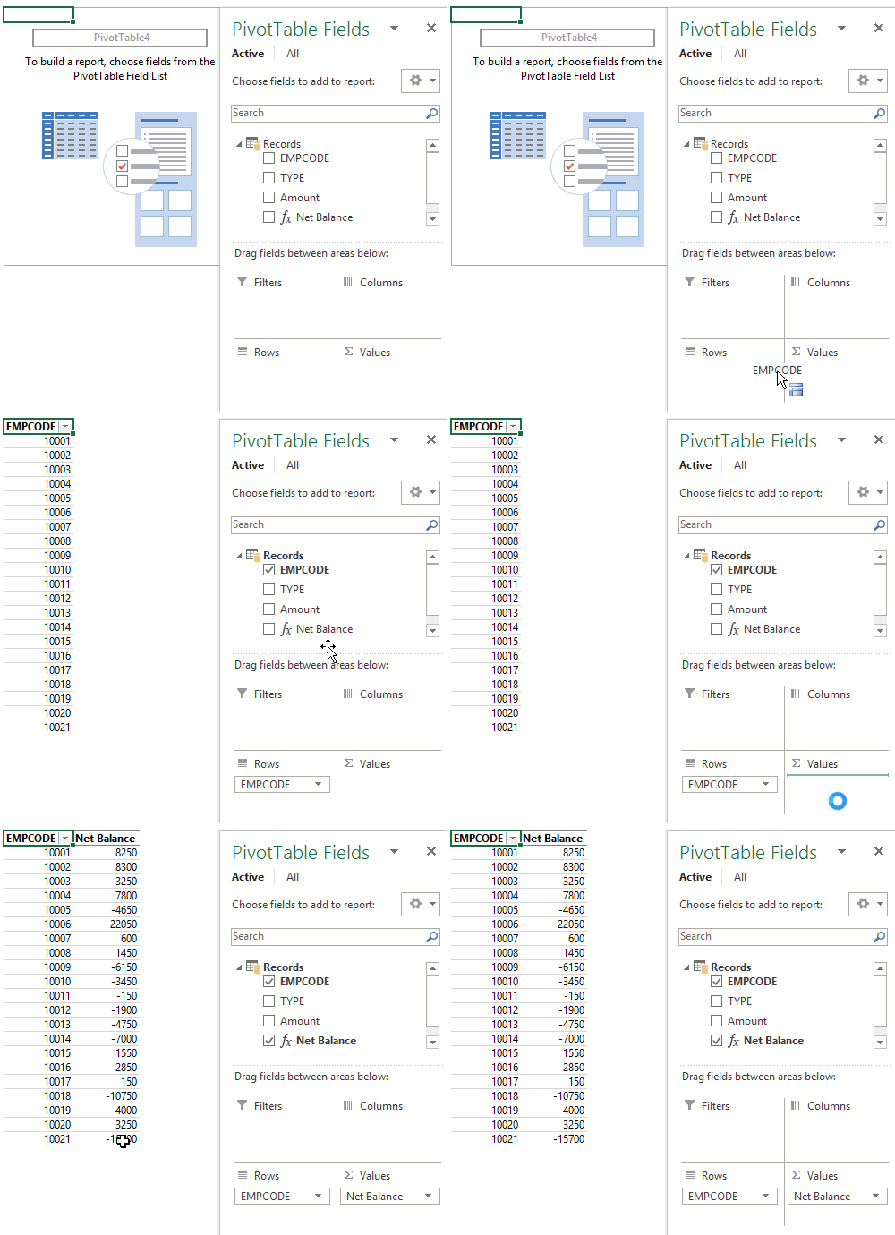
Note the difference that you don’t even have to drag “TYPE” to the Columns area. PowerPivot measures are robust and automatically adjust to the filter context of the pivot tables
