The A-Z of Custom Formatting

 

Is this related to Excel ? Yes Mam it is 😆 !!

This picture speaks miles about what we are going to discuss today.. err.. not a slimming course or anything but how custom formatting can change the way how your data looks like!! 😀

Custom formatting is like a make-up of your data

Guys get your eyes off the picture and lets get started .. shall we? And the I think the best way to start is to tell you that custom formatting does not actually change the underlying data, but only changes the way how it looks! (kept in bold because that is really important and true in most cases)

Ok!! So where is Custom Formatting in Excel ?

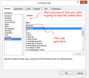
You customize formatting of your data with a code you write in the Format Cells dialogue box (shortcut Ctrl +1) in the custom formatting section

 

Structure & Thumb Rules of Writing a Custom Formatting code

We’ll discuss how to make a code in while but let’s discuss some ground rules first!!

Thumb Rule 1) The custom formatting code can consist of 4 parts

1. The Positive Numbers (1, 4, 100, 5000 etc)
2. The Negative Numbers (-1, -5, -10, -1000 etc)
3. Zero (0)
4. Text (Hi dude, Million, Days etc)

You don’t necessarily need to write the code for all 4 parts. Excel will assume the following in case you choose to omit one or more parts of the code

1. If you writing only the first part –  then it applies to all numbers (+ve, -ve and zeros)
2. Writing only first and second part – then first part formats +ve numbers and zeros and second part formats the -ve numbers
3. Three parts – 1st formats the +ve numbers, 2nd formats the -ve numbers, 3rd formats the zeros

Thumb Rule 2) You have to follow the sequence while writing the code. I mean you cannot write the code for a text first and then for a negative number… it wont work!! So the sequence for all 4 parts of the code will be  Positive Number Code ; Negative Number Code ; Zero Code ; Text Code

Thumb Rule 3) Always separate the parts of codes with a semicolon. Remember the separator is a semicolon (;) not a comma. Simple right?

Thumb Rule 4) Put the text in the code in double quotes, example “Mn”

 

Writing your first code .. a simple case!

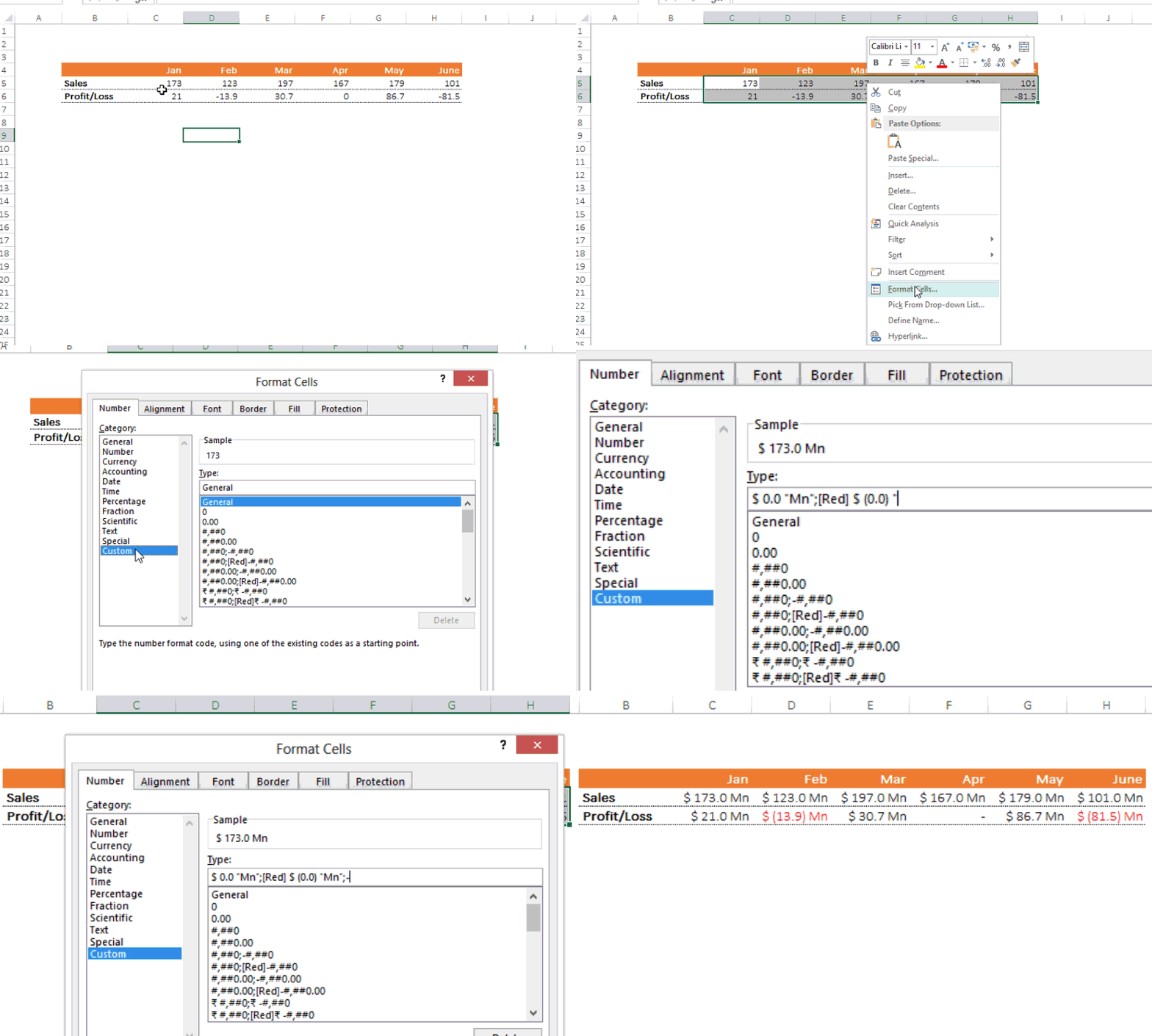
Consider this Sale/Profit data over 6 months

Your boss asks you to format it this way

1. Stacey (even if you are not Stacey 😀 ), all the positive sales/profit numbers should appear this way – $ 173.0 Mn
2. All negative (profit) numbers should appear this way in red color- $ (14.0) Mn
3. All zeros should be replaced with a hypen –

According to the rules our code will follow this sequence positive number code ; negative number code  ; zero code

1. Select your data (numbers only)
2. And go to cell formatting (Ctrl+1) and click custom and start writing the code (by replacing the General)

Code for positive numbers For excel to format any profit/sales number in one decimal prefixed with a $ sign and suffixed with a Mn, we need a variable for sales/profit number.

0 is a variable for any number. So we will write $ 0.0 “Mn”;

Code for negative numbers Now negative number need to be in red and in brackets, rest is the same as positive number coding

Thumb Rule 5) When applying color to any part of the code, make sure the color is written first in square brackets [Red]

So our revised code looks like – $ 0.0 “Mn”;[Red] $ (0.0) “Mn”;

Finally Code for zeros We don’t need to see zeros, instead we want a hypen or a dash so our revised quote looks like $ 0.0 “Mn”;[Red] $ (0.0) “Mn”;–

Note: code is separated with semicolon. Press Ok and see the result in the excel file

 

The positive, negative and zero have been formatted just as the way your boss wanted!  Custom Formatting – Example (download file from down below)

Characters used in Coding

There are whole range of variables and characters that can be used for different utilities in your code

Character	Utility
” “	Displays any text between the double quotes
	Displays the next character as it is
@	Character for displaying any text
*	Repeats the preceding character to fill the width of the cell
#	Displays only significant digits and does not display insignificant zero's, for example it won't display 0001 rather will display 1
0	Displays both significant (non zero numbers) andinsignificant zero's, for example the code 000 will dispay 001,002 and so on
.	Decimal separator shows the number of decimal places after the number, for example 0.0 will show insignificant zeros and 0.# will only significant decimal places
,	Comma if suffixed after # or a 0 it divides the number by 1000, for example 0, 'k' will result the number (15000) in 15 k
%	The percentage (%) symbol multiplies the number by 100 and suffixes the number with a % symbol, for example #.0% will result in 12.0%

 

Date & Time in Custom Formatting

Numbers can also be formatted as dates and time using these characters

d	Shows the number of the day
dd	Shows the number of the day in 2 digit places. For example 07, 09, 15
ddd	Shows the day in words. For exampleSun,Mon, Tue
dddd	Shows the day as unabbreviated. For example Monday, Tuesday, Friday
m	Shows the month number from 1-12
mm	Shows the month number in 2 digits for example 01, 02, 10
mmm	Showsthe month as a short word, example Jan, Feb, Mar
mmmm	Shows the month as a complete word, example March, April, September
yy	Show the last digits of the year, for example 2014 will be shown as 14 and 2000 as 00
yyyy	Shows all four digits of the year

h	Shows the hour
hh	Shows the hour in a 2 digit number example 02 or 09
[h]	Shows the total hours, for example a number (2) formatted as [h] will show 48
m	Shows the minutes. Note it only shows minutes if used as time formatting code (hh mm ss) otherwise it shows single digit months
mm	Shows minutes as a two digit number. Note it only shows minutes if used as time formatting code (hh:mm:ss) otherwise it shows single digit months
[m]	Shows the total minutes, for example a number (2) formatted as [m] will show 2880
S	Shows seconds
ss	Shows the seconds in a 2 digit number example 02 or 59
[s]	Shows the total seconds, for example a number (2) formatted as [s] will show 172800
am/pm	Adds am/pm after the time as per 12 hour clock

Adding Conditions to your custom formatting code !

This is a real game changer and alters some of the thumb rules that have been with us this far. In custom formatting you can also apply conditions

if the number is > than 100 then color is red else color is blue

The new rules!

1. The conditions are written in square brackets [condition]
2. If any color needs to be applied with a condition then colors will come first in the code. For example [red] [condition]
3. The sequence of the condition is important – Excel stops reading the code further if the condition is met
4. Semicolon (;) is used to separate conditions
5. You can write 3 conditions at max

Consider this Code

[>=1000000] 0.0#,, “m”;[>=1000] 0.0#, “k”;0

1. Notice the semicolons. 2 semicolons for separating 3 conditions
2. 1st Condition (in square bracket) is checking if the number is more or equal to 1000000. If this condition is met then format the number as 1.0 m
3. 2nd Condition is checking if the number is greater or equal to 1000 then format the number as 1.0 k
4. 3rd Condition is checking if the number is not meeting any of the above conditions just write the number

This is how the code will format the following numbers

5293925	5.29 m
4761090	4.76 m
874911	874.91 k
390410	390.41 k
5246138	5.25 m
4514427	4.51 m
1785909	1.79 m
2802888	2.8 m

 

Now that we have by and large covered custom formatting next I will write some interesting codes. I think it has been a reasonably long discussion, but I really wanted to give you a comprehensive flavor of how this works, I will close here but once again will reiterate that custom formatting only changes how your data looks and not its actual value. Verify that by applying custom formatting and checking the value in the formula bar!!

How often do you use custom formatting and in what ways, please share and comment!!

Take Care!