A Primer on the INDEX Function !

Versatile, Robust, Fast, Simple, Elegant .. oh all that is ME 😆 and The INDEX function too. Since you already know me so let me introduce you to the INDEX function

 

 Ladies & Gentlemen here is INDEX

If you have been using VLOOKUP for a while, it is time now to graduate baby! Let’s start simple with the Syntax =INDEX(array, row_num, col_num)

1. Array is your lookup range. Just like your vlookup range!
2. Row_num is the row number that you want in your array
3. Col_num (optional) is the column number that you want in your array
4. Assuming all the values fed in correctly the INDEX returns the intersection of row and column number in the array. Trust me it is that simple 😎

 

A Case with INDEX

We have here 5 months sales data of different employees (Emp ID) and we want to look up for EMPCD 255 in March

Aahaa, it is simple VLOOKUP thingy! But let’s get this done with INDEX

Notes

1. I specify the array in which I have to lookup (B3:G95)
2. Row number is 3 for EMPCD 255
3. And Column Number is 4 for March
4. The INDEX returns the value 255 i.e. the intersection of Row and Column number

Ok no rocket science here, this is as good as doing a VLOOKUP! Agree?

 

Let’s get more Interesting in the Case

The same data but now we need the total sales of 5 months for EMPCD 416, of course using the INDEX function. Tricky Huh? You can do this using =SUM (by adding an adjacent column) but my point is how can you extract all values in a row

An additional feature of INDEX is that If you leave the column number empty, it picks up all the values in the array and vice-versa. Check this out..

Notes

1. Array remains the same (B3:G95)
2. The row number for EMPCD 416 is 2
3. And I have skipped the column number (alternatively you can also write 0) This would give me all the values in the row number 2
4. The reason why the INDEX gives you the #VALUE error is because INDEX has pulled out all the values {“EMPCD 416”,675,113,416,175,192} from row number 2, that is exactly what you wanted by but default a single cell can store only one value not 5, so the #VALUE error
5. So we take those 5 values and wrap it around the SUM function. Get it? 😎

 

Another perspective could be asking the total of Feb for all Salesmen (Emp ID)

It is simple: When we left the column number empty it gave all values in the row. We now will leave the row number empty and it will give all the values in the column. Check it out..

Notes

1. Array is the same (B3:G95)
2. Row number is left empty, this will give us all values in the column for Feb
3. Column number is 3 for Feb
4. Wrap that around the SUM function and we have a total of all values in Feb Column

 

Let me impress you more with INDEX, the range maker!

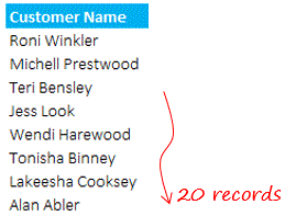
There could be two cases for far. You are impressed or very impressed 😆 but I have more!! Let’s carry on. You can use INDEX on either side of colon : to create a range. Here is quick case on 20 customers mentioned in the list

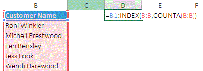
If you have to form a range for these 20 customers you’ll write =$B$1:$B$21, but what if you add two more names in the end and you want the list to dynamically update itself. Here is a solution with INDEX

Notes

1. The first part of the range is fixed at $B$1
2. We are using INDEX to find out the last filled cell in column B
   • The array is entire column B:B
   • The row number is the count of the number of items in Column B. COUNTA(B:B). Assuming that there are no empty cells in the customer list
3. You can use this formula in the named range and the range will change dynamically when names are added or deleted off the list

Read more on INDEX

1. The Imposing Index from Daniel Ferry
2. 7 reasons – Why should you use Index ? from Chandoo

 

How did you find the INDEX ?

Well there is a lot more to INDEX function (where you can lookup in the multiple ranges) but we’ll keep that for another sunny day. Have you used the INDEX before ? Share your experiences

 

Download The Ultimate VLOOKUP Guide

The guide contains tricks and tips beyond the conventional VLOOKUP and it’s free – DOWNLOAD THE ULTIMATE VLOOKUP GUIDE (pdf)