Formatting Tips for Pivot Tables

If you are a data jockey, you would agree with me that Pivot Tables are simply awesome! And under the hood of that awesomeness there are a lot of nick nack features (especially formatting ones) that make pivots even more awesome.

Let’s explore a few of these today!

Tip #1 Turning Off GetPivotData

Often you might find yourself writing formulas outside of the pivot table and that dirty GETPIVOTDATA thingy that pops up when you refer to a cell in a pivot table. You might have found a manual work around to this but here is how you can turn it off

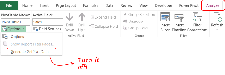
1. Select the Pivot and got to Analyse Tab
2. Under the drop down for Options turn the GETPIVOTDATA off
3. You’ll now forever be able to write formulas without GETPIVOTDATA bothering you

 

Two more things..

1. GETPIVOTDATA is not that bad. I have put it to a great use while building dashboards. May be that topic is for another post
2. DAX formula language in PowerPivot helps you to write (measures) formulas inside the pivot rather writing them outside

 

Tip #2 Convert Pivot Into Tabular Format

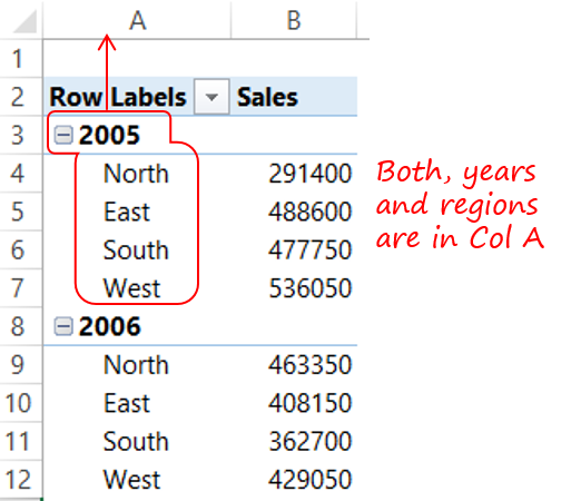
Converting the Pivot into a Tabular Format will separate out the years and regions in 2 different columns. This is something that people usually achieve by Classic Style Layout, which I don’t suggest using

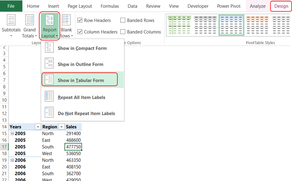
1. Select the Pivot and in the Design Tab
2. Under Report Layout choose Tabular Format

 

Tip #3 Repeat Item Labels

At times you feel the need to repeat the Row Labels across the pivot table (esp for long pivots)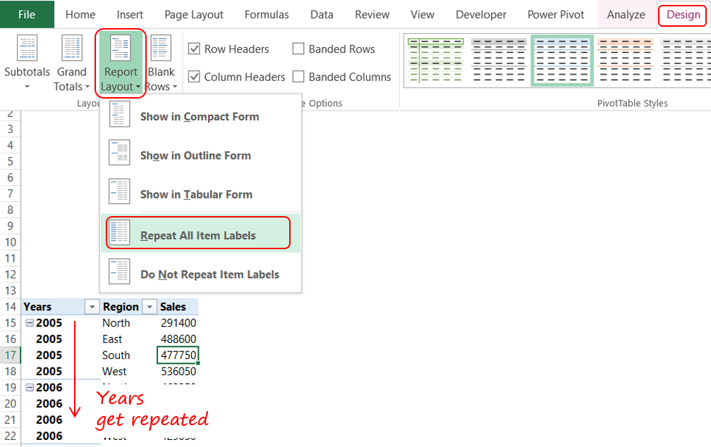 

1. Select the Pivot and in the Design Tab
2. Under Report Layout choose Repeat Item Labels

 

Tip #4 Remove the Plus/Minus (expand/collapse) buttons

Often when you add more than one field under Rows in a Pivot you’ll get a pivot table with Plus Minus buttons, essentially used to expand or collapse parts of the pivot table. Here is how you can remove them

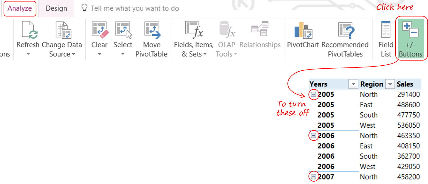
1. In the Analyse Tab
2. Click on the Plus/Minus buttons to turn them off

 

Tip #5 Hide or Display Subtotals and Grand Totals

You may choose to have or hide Sub Totals or Grand Totals. The design tab gives you multiple options to display Grand Totals and Sub Totals

 

Tip #6 Hide/Display Field Headers

If in case you want to remove the pivot table field headers, you can do it this way

 

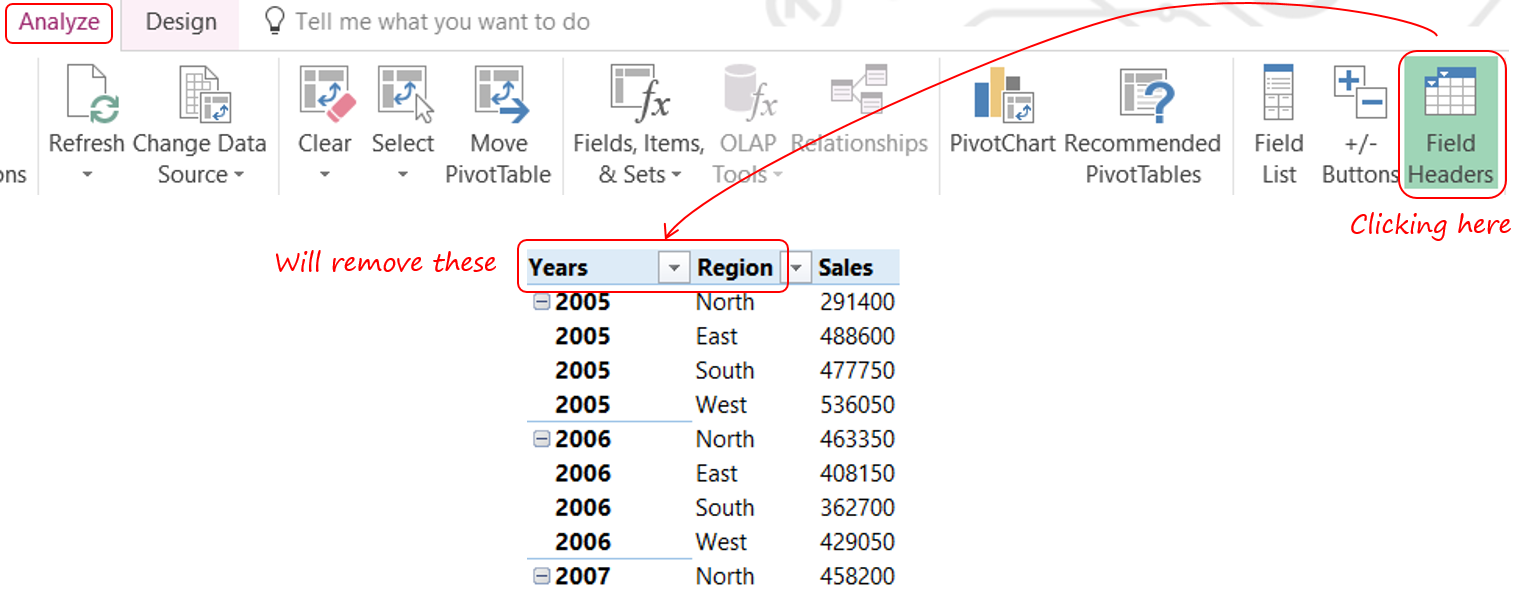
Tip #7 Pivot Table Styles (& my favorite)

Although Pivot Table’s Design Tab offers many different types of styles (look and feel) but I prefer no styling options. So I always go for None (well that’s a style name). It is neat and clean

 

Tip #8 Turn Off Auto Adjust Column Width

When you are constantly shuffling fields (from rows to columns or in values) the column width changes automatically to fit the contents in the cell without wrapping it.

Although this is a good feature but I don’t find this to be helpful when my pivot tables are directly placed in Dashboards. Why..?? because this would constantly alter my screen width

So I turn off the auto fit option

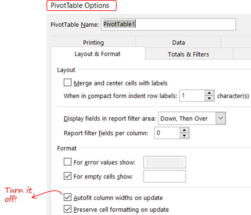
1. Right Click on the Pivot go to Pivot Table Options
2. Under Layout turn off the “Autofit column width on update” option

 

Tip #9 Selection and Moving Pivots

I find these options incredibly helpful to move and select large pivot tables (by large I mean too many row / column fields). There are two options to select (the entire pivot or parts of it) and move the pivot table in the Analyse tab

 

Tip #10 Formatting Empty Cells in the Pivot

In case your Pivot Table has any blank cells (for values). You can choose to customize their display

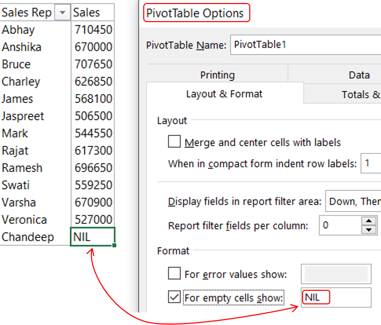
1. Right Click on the Pivot and go to Pivot Table Options
2. Under Layout & Format Tab --> For empty cells show: “NIL” (you can customize this)

 

Tip #11 Custom Sorting of Row / Column values

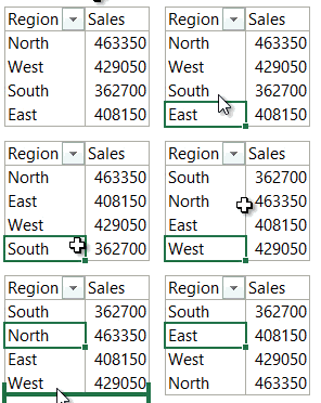
This happens a lot. The default sorting order of row or column (text) labels is A-Z or Z-A. Now there are 2 ways to sort the values in a custom order

1. You can define a custom sorting list in Excel and pivot table will then automatically adjust to the custom list
2. Move row/columns labels manually with the mouse

 

Tip #12 Sort the Field List

This one is pretty straight forward. Sorting the field list helps especially if you have too many columns in your data.

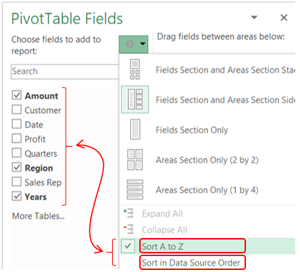
1. Click on gear icon in the field list
2. And choose the sorting option

 

Tip #13 Insert a Blank Line after each Item

This one is more used from a hygiene perspective.

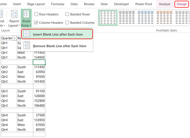
1. From the Design Tab
2. Under Blank Rows --> You can choose to add or delete a blank row after each item

 

Tip #14 Filtering Values in Pivot Tables

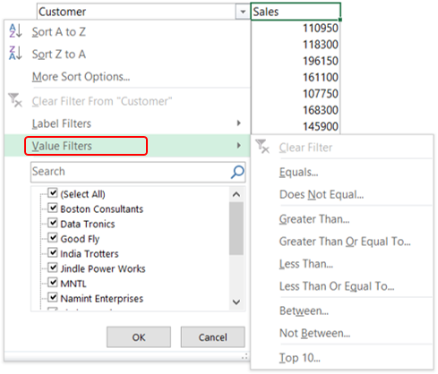
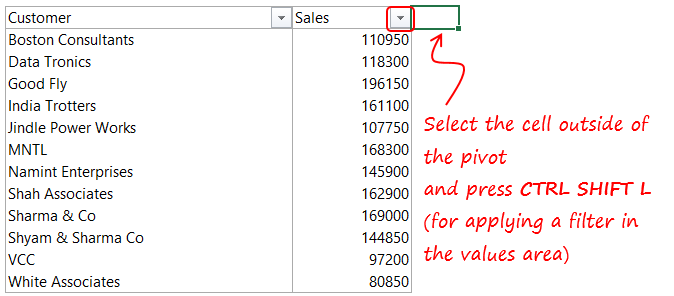
You must have seen filters for Row / Columns items but not for Values. Well the filter buttons are missing from the pivots. Here are 2 ways to get it

Method 1 : Is by choosing value filters in the filter drop down of the row labels

 

Method 2 : Selecting the adjacent cell outside the pivot and press CTRL SHIFT L. This will directly give you a filter on the Sales Values

 

Tip #15 Disable Drill Down

Double click on the cell inside a pivot table gets you its source data. You can disable that from Pivot Table Options

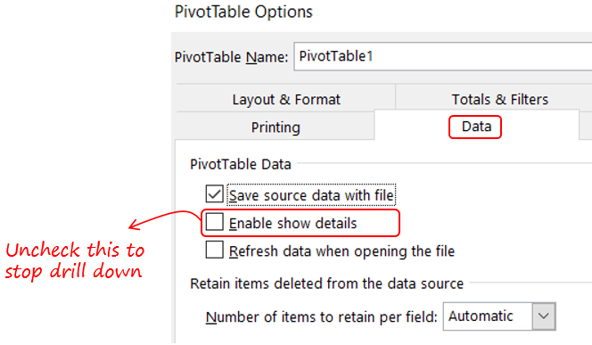
1. Right Click and go to Pivot Table Options
2. Click on Data Tab and
3. Uncheck ‘Enable Show Details’

Note that the user can turn this back on, so you might want to protect your sheet before sending it

 

Do you have any more formatting tips?

Please drop in a comment in case you have some regularly used formatting tactics for pivot tables.

 

Some More Pivot Hacks

1. Take a Short Pivot Table Course – it’s free
2. 16 Pivot Table Tricks – to improve your efficiency
3. The correct way of applying Conditional Formatting in Pivot Tables
4. Change Pivot Table Value Calculation – using VBA