Have you ever had a situation where you wanted to inverse the order of your data? .. If yes then this is just for YOU! Read on..
The Situation
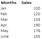
We have a small data set for 6 months Sales (Jan – June). Please note that the months (Jan, Feb .. are not dates they are just text values). We want to inverse the order here and we are certainly not going to cut/copy paste each value and change the order.. lets do something more automated and smarter! Ready?

The Formula

Done!! 
Lets take a deep dive into the formula !
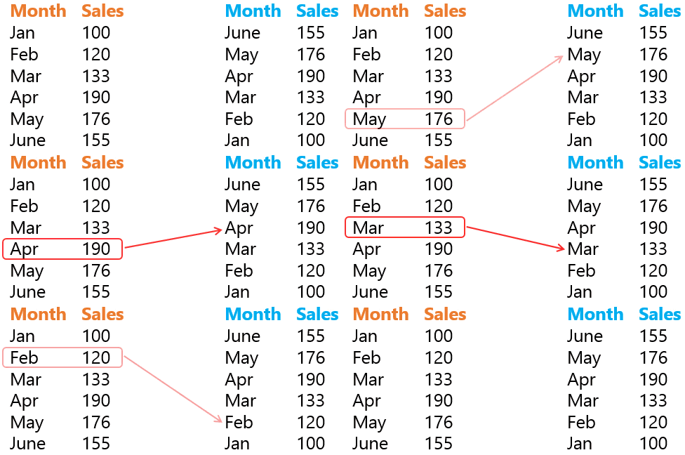
Take a look at the logic first

So there are 2 parts in the formula the INDEX and the ROWS. Lets tame the ROWS first
- =ROWS(B4:B$9) will do two things
- It will return the number of rows in the selected array, so from B4:B$9 there are 6 rows
- When formula is copied down it shrinks the array because we have locked the row 9 (B$9) so as it moves down it returns the numbers 5,4,3,2,1 [Learn more on Cell Referencing and Tricks]
- =INDEX($B$4:$C$9,ROWS(..),1) – Since we have already discussed the ROWS formula we skip it here
- $B$4:$C$9 defines the array where we want to do a lookup
- The ROWS is extracting the row number
- 1 in the end is the column number
- So when we want extract the sales, we copy the same formula and change the column number to 2. (You can make it more sophisticated with the MATCH Function, but we’ll reserve that part for some other day)
Subscribe for more Tips and Tricks
I be happy to send you a quick mail as and when I post something interesting and trust me it is absolutely effortless learning a tip once in a while.. actually is fun! Fill in your details in the subscribe box in the right panel … see ya in the next one, take care!
