Leave Data Analysis using Power Query – Case Study

A few days ago, we (Abhay and I) did a webinar on Power Query. As a sample we picked up an interesting set of junk employee leave data and showed how to transform that in Power Query. In case you missed attending the webinar, you can catch up with the learning in this post

The tricks shared in this post can be applied at a lot of other places as well. This post is written by my friend Abhay Gadiya (power query prodigy)

Let’s dive in! Enters Abhay >

Assume the HR department keeps track of leaves taken by employees in an Excel sheet something like this

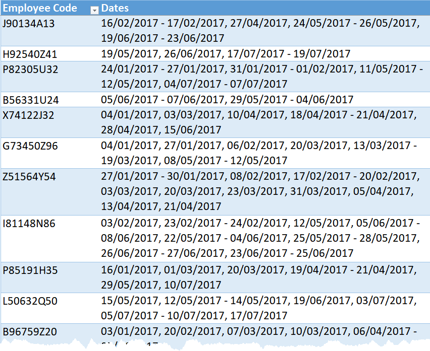
You can notice that leave data for each employee is stored in single cell, in a single row under 'Dates' column. It is separated by comma and multiple leave dates are separated by '-' hyphen

Using this data how will you answer these questions

1. How many leaves each employee has taken till date?
2. Are there any specific days in a week when many people are taking leaves?
3. Are there any specific days in a month when many people are taking leaves?

With current structure of data it is impossible to answer these questions. You need to have data in structure something like below

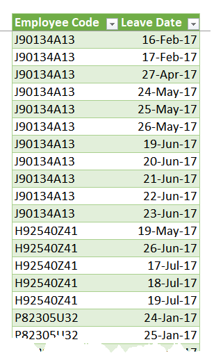
Here on each row we have single leave date for each employee. Let’s see how can we achieve this using Power Query

 

Let the Data Cleansing Begin..

First step is to simply load the data into Power Query. To do this select any cell inside the table and then go to Data > From Table.

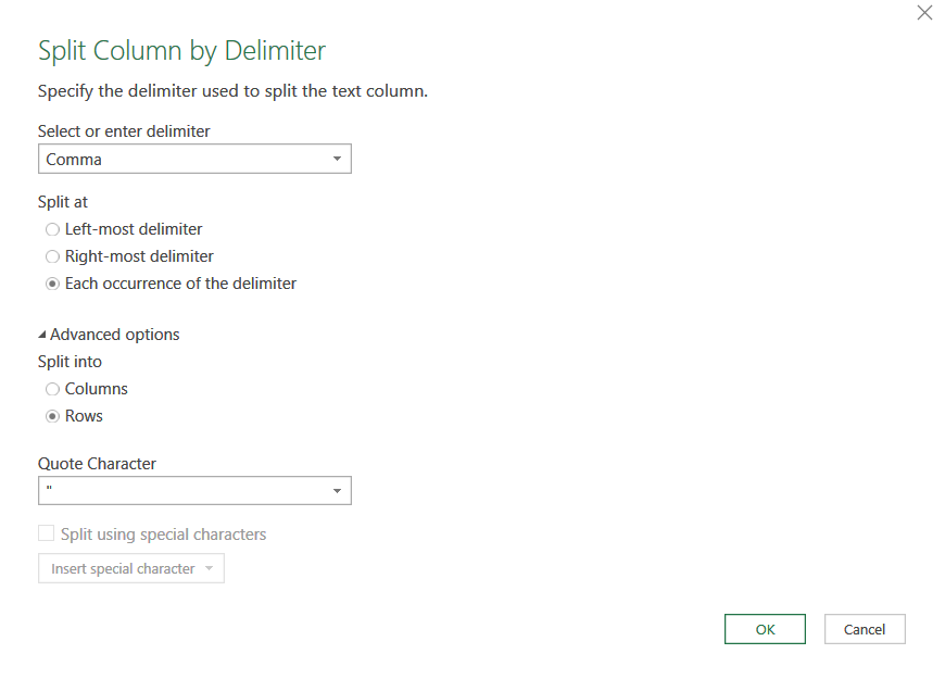
Next select Dates column and then go to Split Column > By Delimiter. In new window opened select 'Comma' as delimiter and at each occurrence of the delimiter. Under advanced options select 'Rows' and click OK.

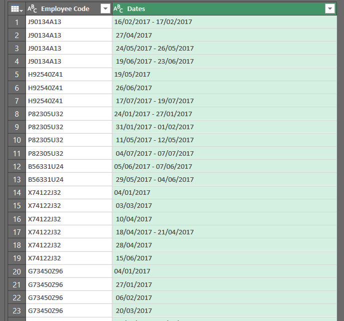
You’ll get an output something like below, where each employee’s leave data is split in rows from a single cell. This functionality is different from normal text to columns inside Excel

Now we need to split dates column one more time using '-' as delimiter and using 'Columns' from advanced options. This time we have separated the data from a single cell into two columns and it is very similar to text to columns. Your output should appear like this

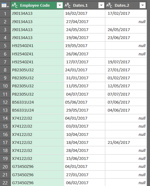
As next step we need to get series of dates between dates stored in above two columns. e.g. in third row we have 24/05/2017 under Dates.1 column and under Dates.2 26/05/2017 column. Here we need to get date in between dates as well which is 25/05/2017 for this row. We will have to get this for another row as well

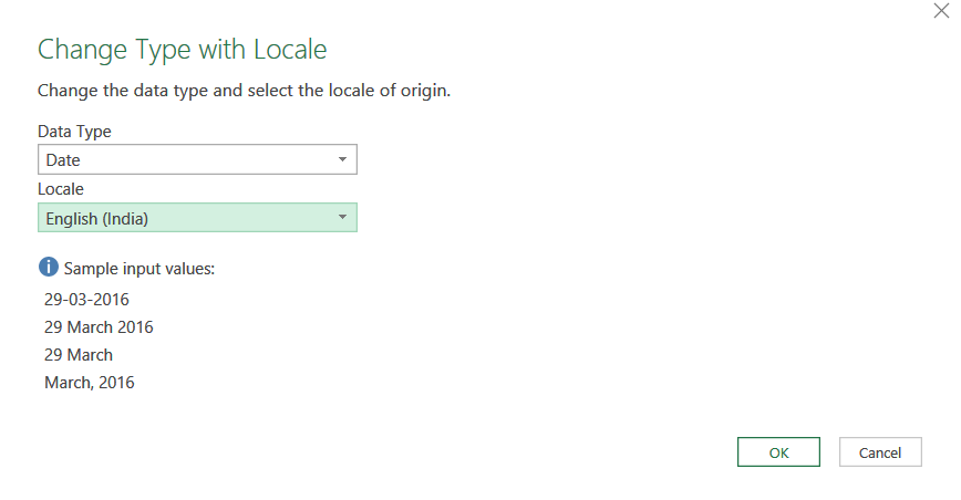
To get this first we would need to convert these columns in date format. So, we will simply select these two columns and right click > Change Type > Using Locale.

Then we will select Date and English (India) in a new window opened for transformation like in below screenshot

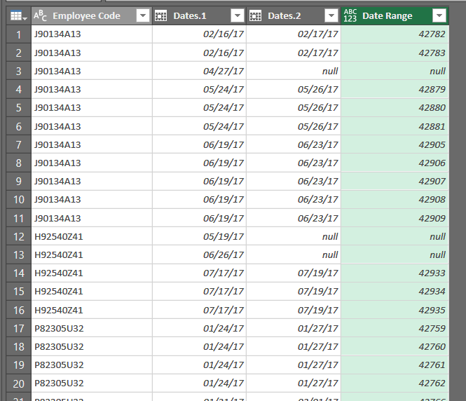
This will convert data in above columns into dates. Now we will insert a new column through Add Columns > Custom Column. We will insert following formula in this custom column window:

This will add a new column with list of dates between the start and end date mentioned in above formula by referencing to Dates.1 and Dates.2 column respectively. You’ll will get the data transformed like in below screenshot:

You’ll will have to then click on double headed arrow in the Date Range Column you’ll then get individual dates in single row like below

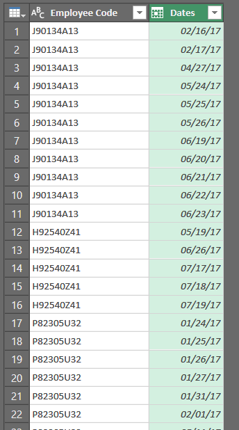
Now we need to combine these three dates column into one. Wherever there is null value inside Date Range column you should pick value from Dates.1 column else keep the value from Dates Range column. Just as above you can do this using custom column window and if function

Now you can remove other columns and simply keep Employee code and Dates column. Change Dates column data type to Date. Finally we have got the data ready like the way we wanted it 😀

You can then load this data back to Excel sheet and can start performing analysis using Pivot tables. However, you can also automate that analysis inside Power Query itself.

 

Let’s try to do this via Power Query

Right click the query and select duplicate like in below window. Do it twice to create two new queries. Rename them as well

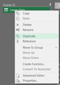
Renamed queries are 'Day_Month' and 'Weekday_Month'.

Since these are duplicate queries all the steps from original query will get copied and these will be independent queries. These will not have any inter dependencies between each other.

Now select Day_Month query and then select 'Leave Date' column.

Go to Add Columns > Date > Month > Name of Month. This will add a new column with month names.

Do it one more time for day, add columns > Date > Day > Day. This will add a new column with day from the dates.

Once these columns are added you can then remove the Leave date column.

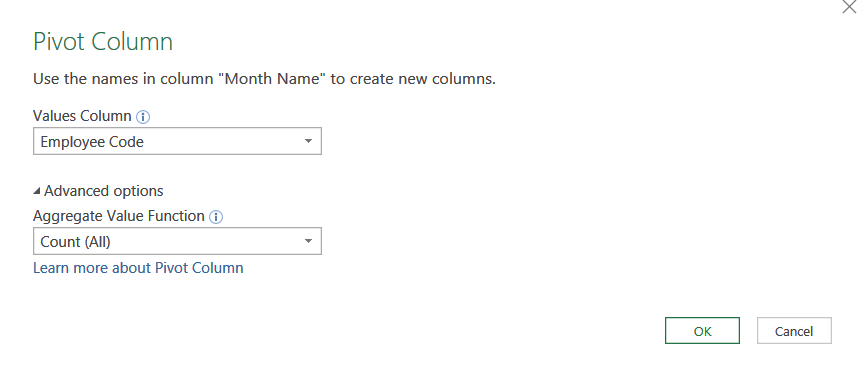
Then select month column and go to transform tab > Pivot Column.

A new window will open up. Choose the options as shown in below screenshot and click ok

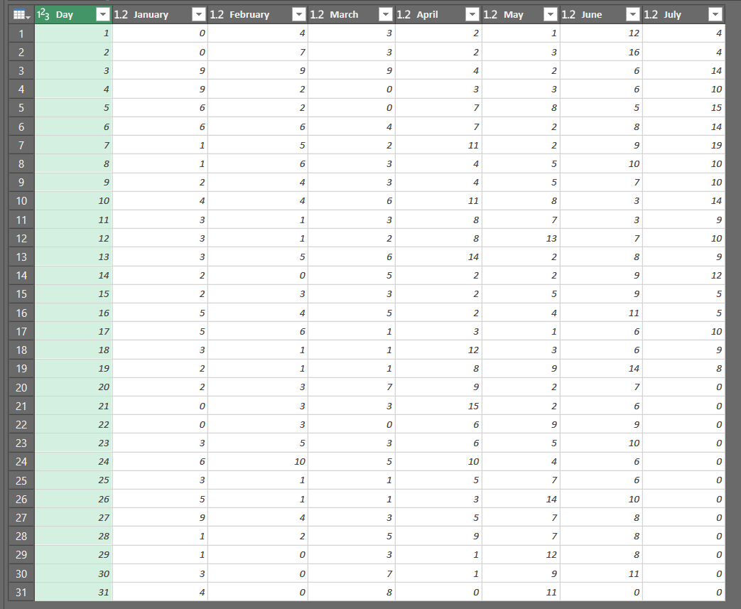
You will get data in following format. You can rearrange the column to display it as shown below:

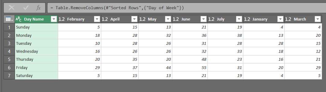
Now, select Weekday_Month query and similarly get Month, Day Name, Day of the week from date column.

Once you have that you can remove leave date column and Pivot month column similar to above.

You can then sort the data using weekday number column and then remove it.

Finally, you will get following data:

Now, you can simply close and load data from above queries back to Excel sheet.

If any new data is being added or existing data has been modified then you should simply click Data > Refresh All to get output updated with latest data

 

In case you understand better by watching.. enjoy!

 

More Power Query Tutorials

1. Perform Vlookup in Power Query
2. Combine Duplicate VLookup Values in a Single Row
3. Merge Data from Multiple Excel files in a Single Workbook
4. Repeat Row N times

 

Become Awesome in Power Query

If you want to be a data superhero. You must consider learning power query from scratch. Consider enrolling in our Step by Step Power Query Training