Ever wondered how to trick VLookup ?
This is simple!
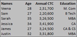
1. Select the entire range

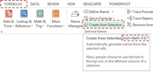
2. Go to ‘Create from selection’ in the Formula Tab or use the shortcut Ctrl + Shift + F3. I recommend to use the shortcut.. its much faster that way 😀
You’re Welcome!!

3. The names are kept in the Top Row and the Left Columns, make sure that both are ticked. Click OK.. and now the real fun begins

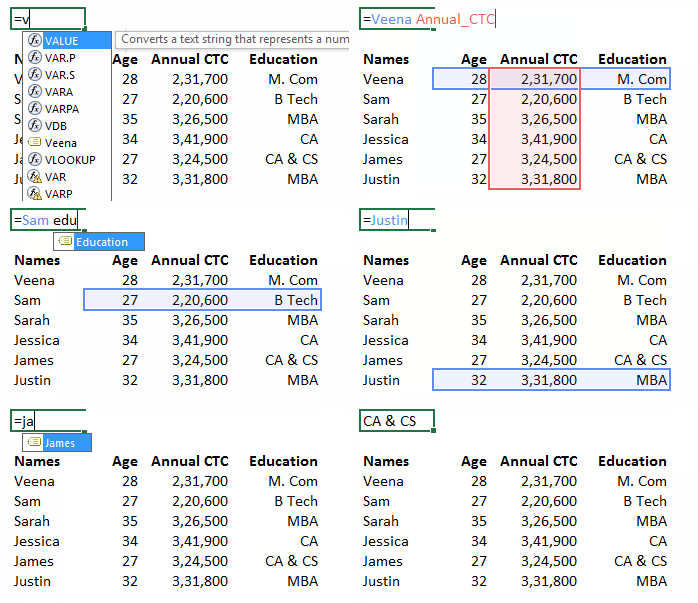
4. Now simply type in the name and the category with a space in between. Yeah that’s the trick, the space actually creates an intersection between the named ranges and allows you to extract the intersecting value
5. Suggestion: Don’t use this trick for heavy data sets. Large named ranges may slow down excel’s processing speed or it may crash. Although its cool to use it for smaller data sets but with large data stick to our very own VLookup/Index/Match functions
Learn More on Cell and Range Naming
Cheers and Take Care!!
