Here is a Quick Tip to generate serial numbers
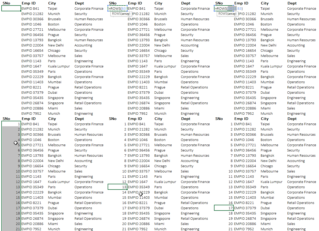
The ROWS Function gives you the numbers of rows in a selected range of cells, for example =ROWS(A1:A10) will return 10 and =ROWS(B5:D20) will return 16. The trick is to lock the first part of the range (=$A$4)* so when you drag the formula down the range expands. Read more about cell referencing and expanding arrays
* note that I have applied absolute referencing here, you can also only freeze only the row i.e A$4 (press F4 two times)
An alternative way – The ROW Function
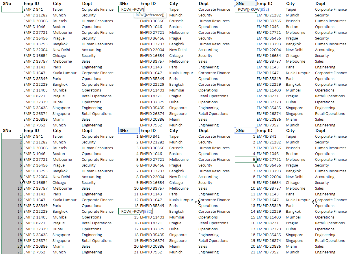
This can also be done with the ROW function

=ROW(A1) returns the row number of the cell A1 i.e. 1 if you just write =ROW() and do not refer to any cell it will return the row number of the cell in which you write the formula
The trick is to take a difference between the current row =ROW() and the header row of the data =ROW(B$2) and freeze the row reference. Now when you drag the formula down the =ROW() will return current row number minus the header row number =ROW(B$2) that will generate serial numbers
The good part about this trick
In case you happen to add or delete any row in between your data the row numbers will update automatically. In case you are adding a row you just have to copy the formula to the new row. Isn’t it cool 😎
See you in the next one!! Take Care
