Scrolling list in Excel

Presenting an elegant solution to displaying large data via scroll-able list. All you need is a

• Scrollbar,
• A list (of course)
• And formulas to tighten everything together !!

Lets make a killing here

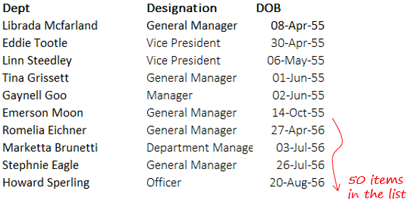
So here is our list!

We have 50 Employees with Designation and Date of Birth (Download the list)

Next we need a Scrollbar

You’ll have to buy one! 😯 .. Just kidding 😆 You will find the scrollbar in the Insert drop down in Developer tab (can’t find Developer Tab ? Read here !)

• Click on the Scrollbar and draw one on the sheet, keep the orientation vertical (it can be drawn both ways, vertical and horizontal)
• Formatting the scrollbar
  • Right click and go to Format Control (alternative shortcut is CTRL 1)
  • Set the Minimum Value to 0
  • Maximum Value to 40 (because we have 10 empty rows between the top and bottom end of the scrollbar)
  • Link it to a cell in the sheet. Now when you shift the scroller, you’ll see the linked cell reflecting the value as per scrollbar’s movement

Tying everything together with a formula

The Logic goes like this

1. As we move the scroller the value in the linked cell changes.. right?
2. From that number (in the linked cell) we want 9 more rows to be displayed between our scroll bar.. with me till now?
3. We will use the INDEX formula to lookup the values in the main employee table

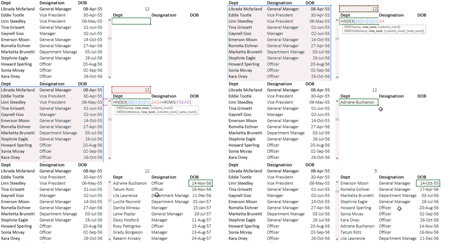
Here is our formula =INDEX($B$4:$D$53,$G$4+ROWS(F$6:F6),COLUMNS($G5:G5))

Decoding the formula 

• The Index function is looking in the array of the employees $B$4:$D$53
• The row number is the Linked Cell + Row Incrementor .. Why? because we want 9 more values after the linked cell. [Related: Learn how to make a row incrementor] $G$4+ROWS(F$6:F6)
• Column number is displayed by the column incrementor because when we copy the formula to the right we need to display the next column result COLUMNS($G5:G5)

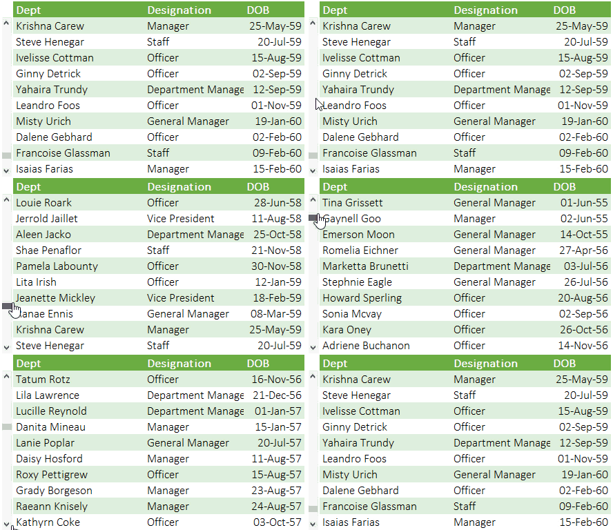
Here is a quick snapshot

More applications of the scrollbar

How to make a stock ticker chart