Calculated Fields in Pivot Tables – A Case

One of the less known and extremely awesome feature of Pivot Tables is its ability to create calculated fields with in the Pivot Table

Take a look at this case!

 

 

 

 

 

 

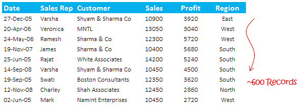
Lets quickly summarize the data in a pivot table with region wise sales, shall we ?

 

 

 

 

 

 

 

 

 

 

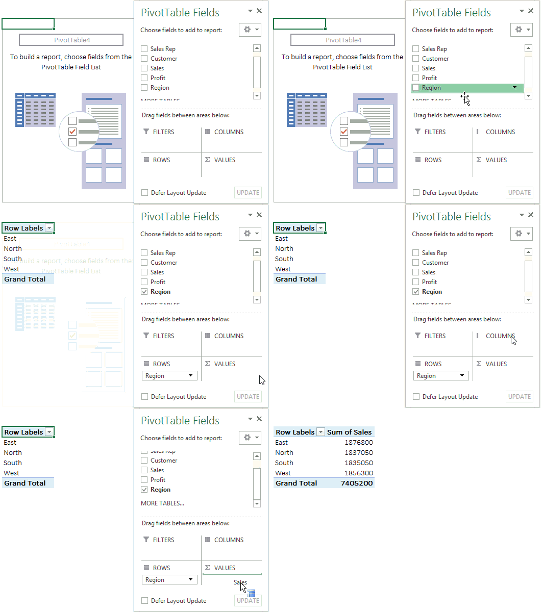
Simple – Drop the Region in Rows and Sales in Values. But what if we have to calculate the profitability region wise?  Don’t mistake the profitability as Sum of Profit. Profitability means Profit/Sales or the Percentage Profit. One of the ways to get this done is through calculated fields

 

Introducing Calculated Field in Pivot Tables

 

 

 

 

 

 

 

(Picture Credit – Mynda from MyOnline training hub)

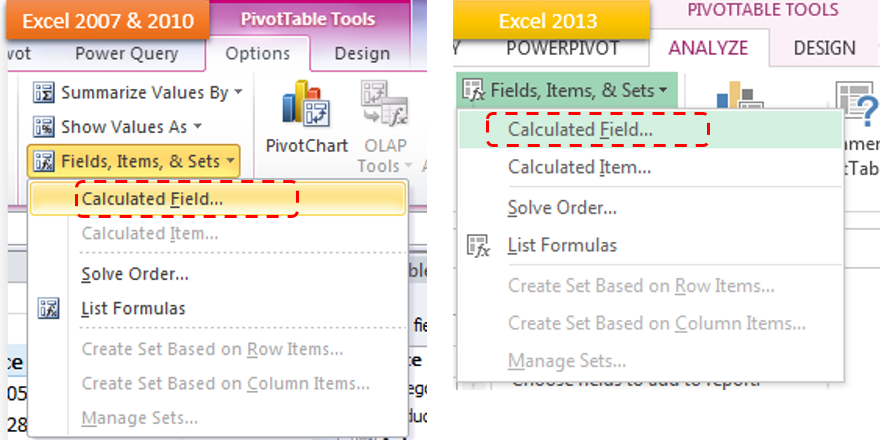
• Excel 2007 & 2010 – Calculated Field is placed in the Options Tab under Field, Items and Sets
• Excel 2013 – Placed the Analyse Tab under Fields, Items & Sets

With this option you can add a custom calculated field in the pivot table. Lets take a look!

 

How to use Calculate Field Option

 

 

 

 

 

 

 

 

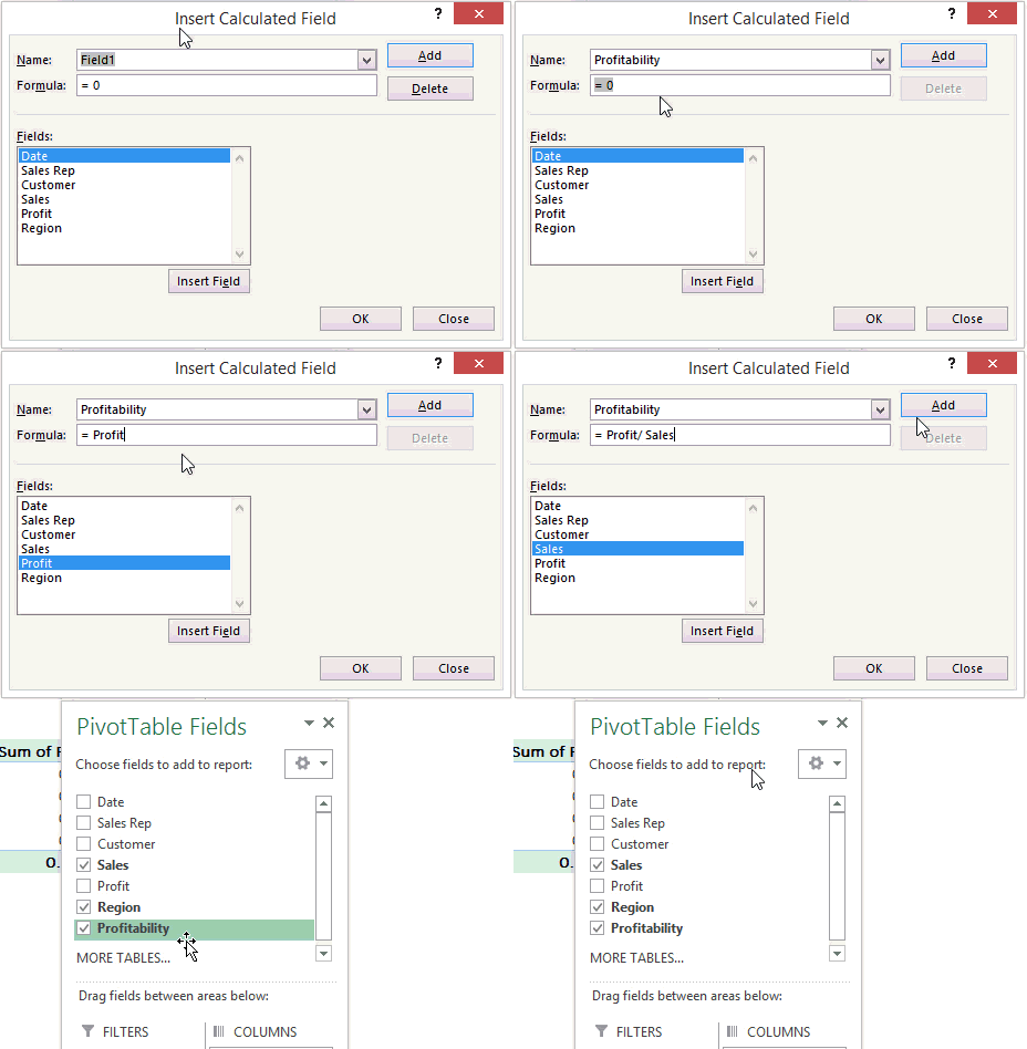
1. Give your calculated field a name. We are calling here ‘Profitability’
2. You can use Functions and Operators (+ , – , / , *) and existing fields to make a customized calculated field
3. Note that you cannot use functions or array formulas that require cell references or defined names. Functions without cell references can be used for example in this case you can also write the formulas as =IFERROR(Profit / Sales, “NIL”)

 

Add the Calculated Field to your Pivot Table

 

 

 

 

 

 

 

 

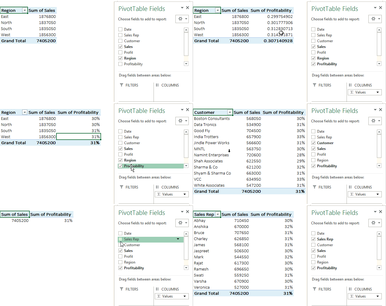
You can use the calculated fields just like other fields. Now you see profitability Region wise, Customer wise or Sales Rep wise

 

More on Pivot Tables

1. Data Models in Pivot Tables – Excel 2013 Feature
2. How to turn off GETPIVOTDATA
3. Grouping Dates into Quarters or Months in Pivot Tables