Know your Charting Arsenal ! (Part 2/3)

After we are done knowing what charts are available in Excel (from Part 1 Chart Arsenal) Let’s just figure out how to do these 2 things

1. Adding / Editing data to your charts

We have a case where we have a pre-built chart for computer sales but we have 2 things missing from the chart. The years on the horizontal axis and the sales of tablets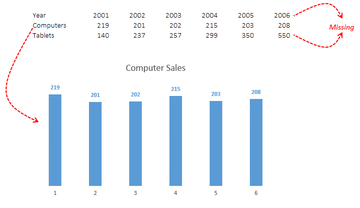

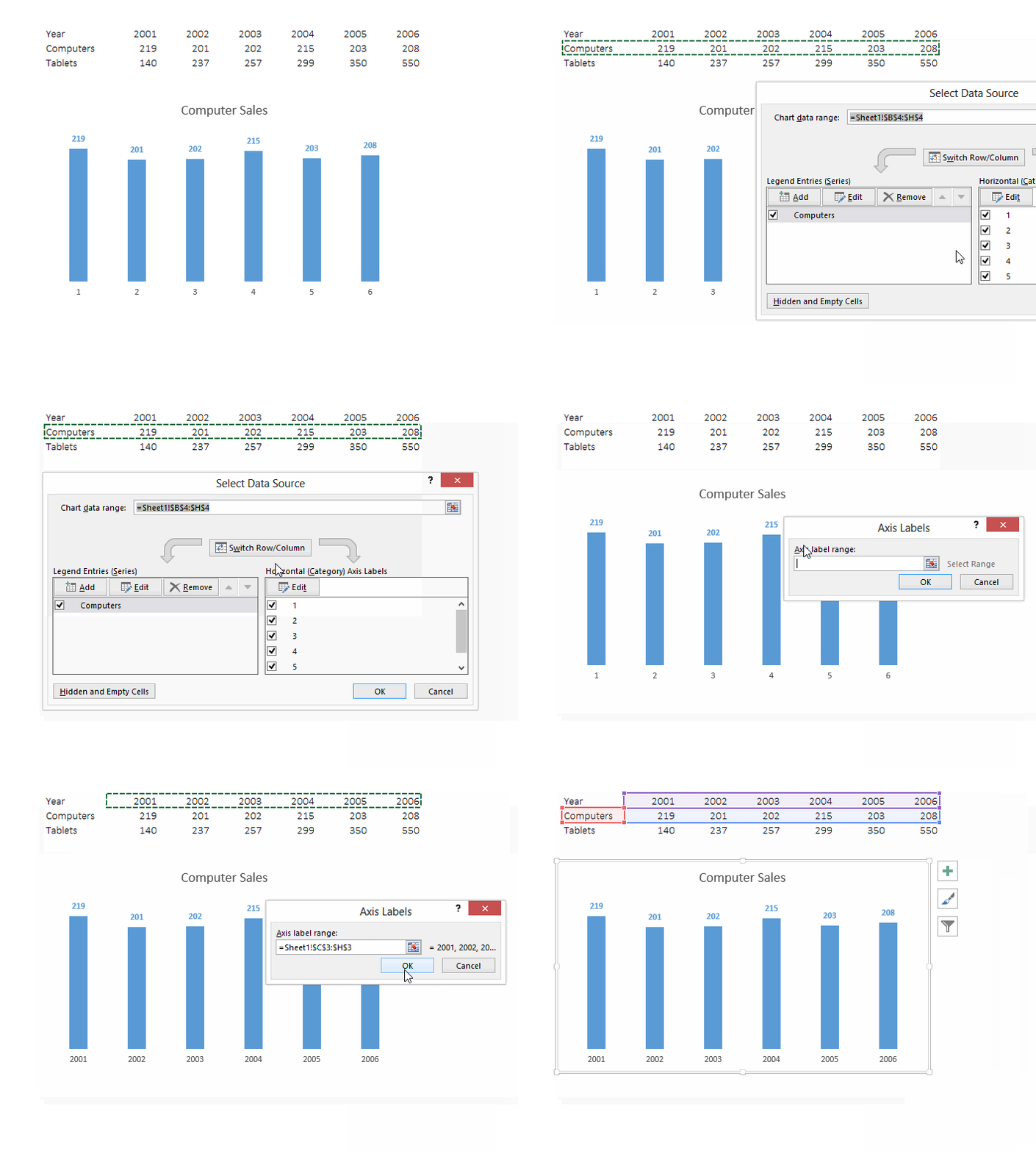
Adding the Years

1. Right Click on the Chart
2. Choose Select Data Option
3. In the Horizontal Axis Labels – Choose the Edit Option
4. And select the year values from the sheet

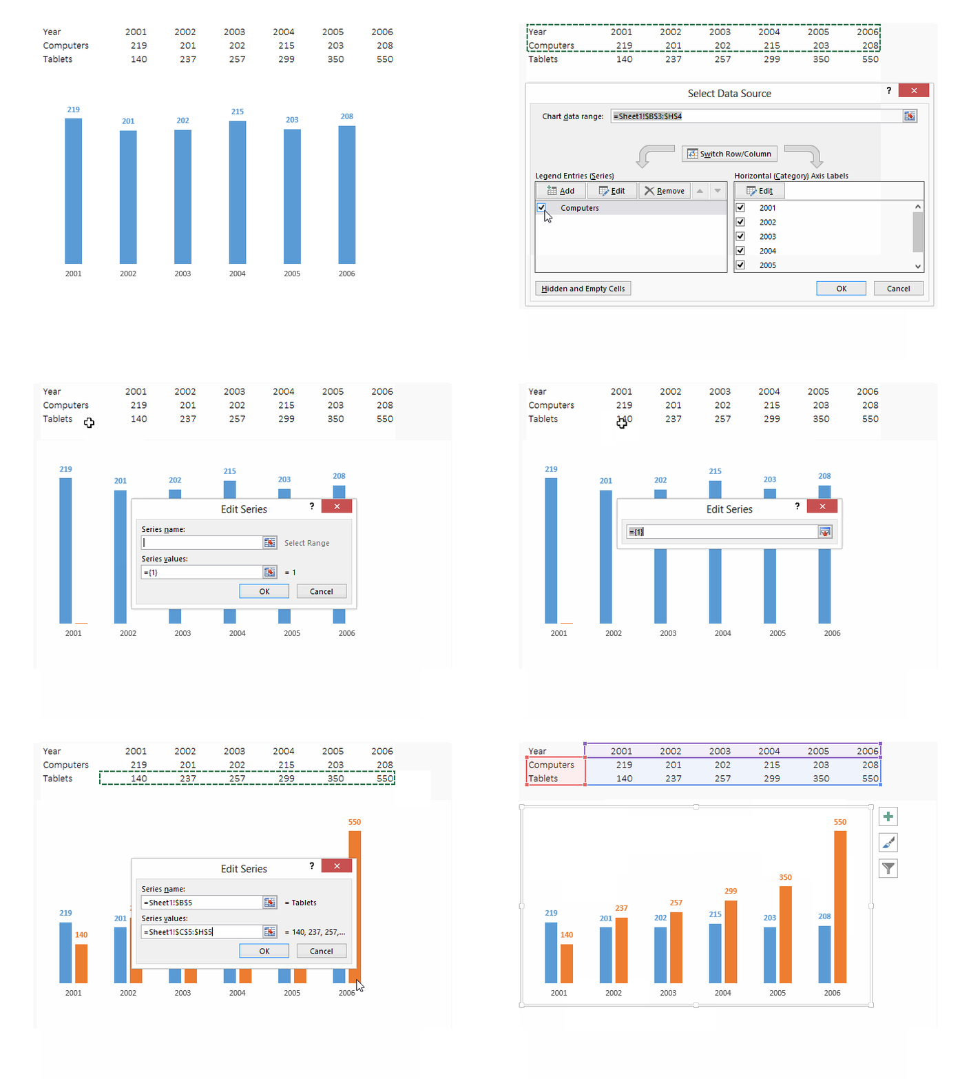
Adding the Tablet Sales

1. Right Click on the Chart
2. Choose Select Data Option
3. In the Legend Series – Choose the Add Option
4. And select the Tablet sales data (name and values) from the sheet

2. Adding Chart Elements

Most Chart Elements like Chart Title, Axis, Legends, etc. often automatically appear when you make a standard chart, but in case you happen to delete them or want to add one or more specific elements then the following are the places to look for

in Excel 2007

Note that

1. The Layout tab is only activated (seen) when you select the chart
2. The Layout tab has the options of adding all the chart elements

in Excel 2013

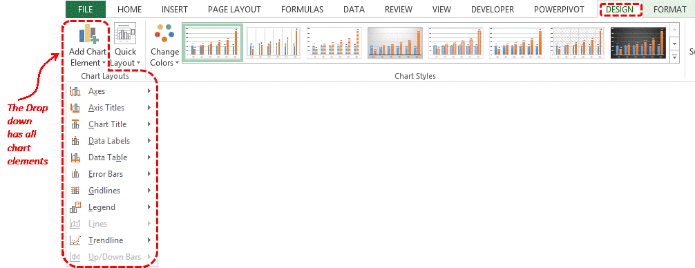
In contrast to Excel 2007 (3 chart tabs), Excel 2013 has just 2 tabs the Design Tab and the Format Tab. The Design Tab has all the chart elements, alternatively you can also click on the + sign  (appears when you click the chart)

Design Tab Snapshot

The Alternative ‘+’ Sign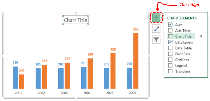

Stay tuned to Part 3 of this series to know about Chart Formatting Options

Take Care!