Create List of Hyperlinked Sheet Names in Excel

This is one of the most common needs while dealing with workbooks with many sheets. And if you have (at any point in time) dragged yourself into the task of manually creating a List of Sheets Names in Excel and then Hyperlinked each one of them, you’ll be ridiculed to see how simple is this task 😀

In this post I am going to show you 2 things

1. How to easily create a list of sheet names (you may also call it index of sheets)
2. And then how to create a hyperlink for each sheet name

And for this we’ll be using a mix of Power Query and Excel Formulas to get it done fast and easy!

 

Imagine a Workbook with Multiple Sheets

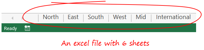
• For this example I am taking 6 but there could very well be 60 sheets
• No order of arrangement and they could be named anything

 

Creating the List of Sheet Names

To be able to do that and make it dynamic (meaning the list should update when sheets get added or deleted) we’ll be needing Power Query. Let’s Load this Excel Workbook into Power Query

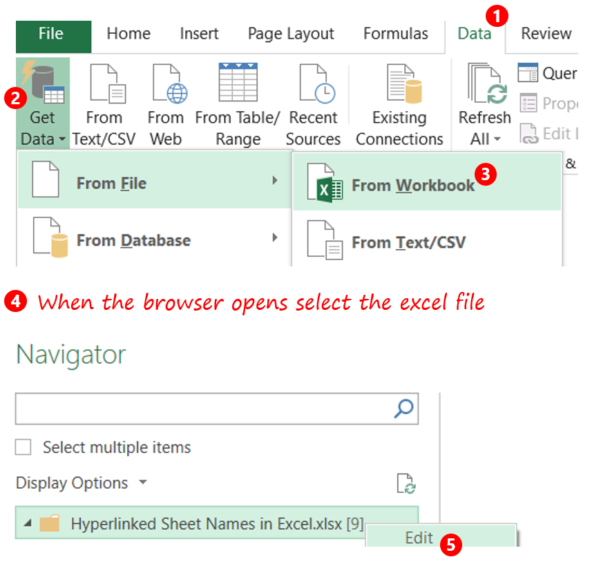
1. In Excel 2016, Go to Data
2. From Get Data go to the File Option
3. Choose from Workbook
4. In the browser window choose the excel file (the file in which you want to create a sheet index)
5. In the Navigator pane right click on the Name of the File and choose ‘Edit’

 

You’ll see the list of all 6 sheets in the Power Query Window

 

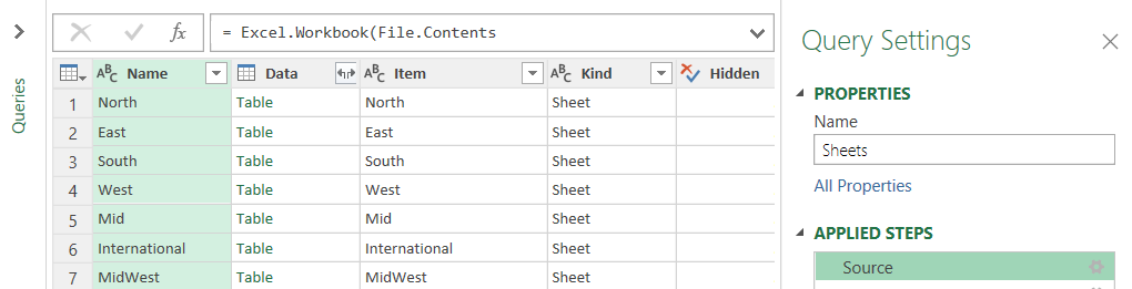
We’ll need to clean the query a bit..

1. Let’s start with applying a filer on the Column ‘Kind’ and select only ‘Sheet’
2. Next Apply the Filter on the Column ‘Name’ and remove the sheet name “Index”. I am doing this because I’ll be calling my sheet “Index” and I don’t want that to appear in the list
3. Just keep the Name column and remove the rest
4. Now simply close and load this query in Excel. You’ll have a nice one columnar table with all the Sheet Names

 

Creating Hyperlinks for Sheets

In the adjacent column of this Table, write the following HYPERLINK formula to create a hyperlink for each sheet

 

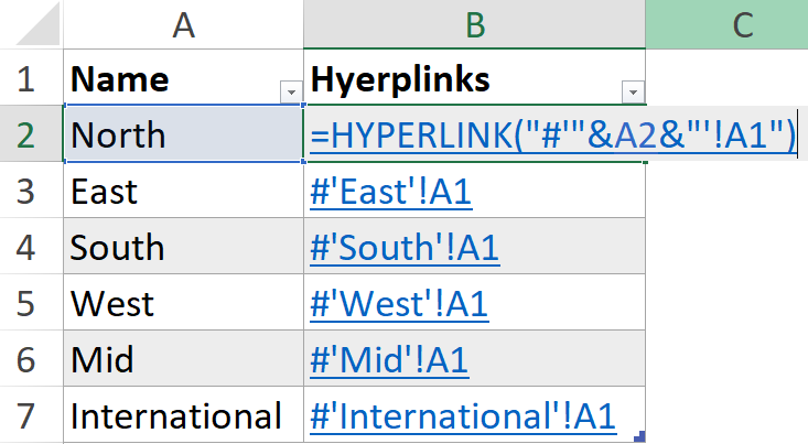
=HYPERLINK('#''&A2&''!A1')

Make sure to take care of the single apostrophes and exclamations, they matter a lot! This formula will pick up each sheet name in Column A and will covert it into a hyperlink to cell A1 of the respective sheet

Also this whole exercise would be sort of incomplete unless we have one more hyperlink on each sheet to link it back to the Index Sheet. Let’s do that as well

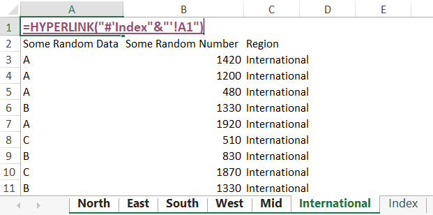
1. Select all sheets but not the Index Sheet
2. Go to Cell A1 (or any other cell where you’d like to create a backward link)
3. Type the following formula

=HYPERLINK('#'Index'&''!A1')

This will create a link back to the Index Sheet on all selected sheets.

 

Is this Solution Dynamic?

Well almost yes!

1. In case you add/delete a new sheet the list and the hyperlink formula will update automatically
2. But you’ll have to manually paste the Hyperlink formula for the Index Sheet into the new sheet added
   • The smart way to do that is to select multiple sheets (in case more than one sheet has been added)
   • Then paste the formula on any one of them and it replicates to each one of them

 

Like Watching Videos Instead? Take a look..

Similar Interesting Stuff

1. Learn how the HYPERLINK formulas works
2. Create a Sheet Index using VBA
3. Hide Sheets that are difficult to unhide
4. Unhide Multiple Sheets at Once
5. Work on Multiple Sheets at Once
6. Consolidate Data from Multiple Sheets using VBA
7. Protect Sheet from being Edited
8. Scroll 2 excel files simultaneously