Transpose Rows into Columns in Excel

Here is a quick problem that I solved for one of our readers a few days ago. This could be a very common scenario for a lot of people, take a look..

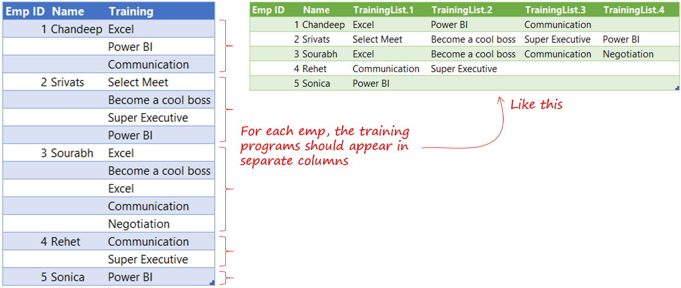
The Table on the left (in blue) contains employee info and training programs for each employee. The task is to transpose each row of training programs into separate columns like the table on right (in green)

Let’s crack this using Power Query

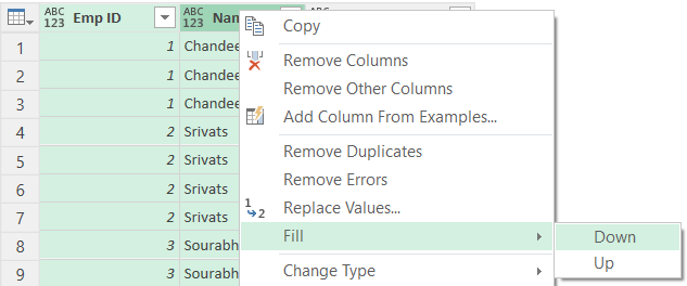
Obviously the first step is to load the data in Power Query. Once the data is loaded to fill the empty rows with Emp Code and Name, select both Emp ID and Emp Name Column in the Right Click menu choose Fill >> Down

Also you may notice that Emp3 has attended “Excel” Training twice in case you want to remove duplicates, select both columns Emp ID and Training >> Right Click >> Remove Duplicates. This is like doing a concatenated remove duplicates

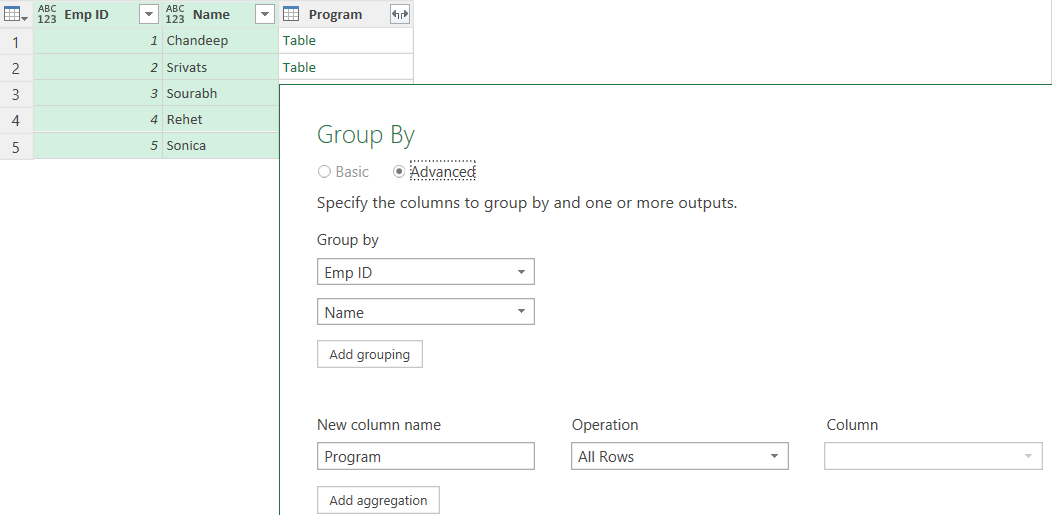
Now let’s group this data by Emp ID and Name. This will let you remove duplicate Employee rows and yet somehow retain the Training information. From the Transform Tab >> Group By >> In the Group By Option Box

1. Go to Advanced
2. Group by Emp ID & Name
3. Create a new column “Program” (it could be any name) and set the Operation as All Rows
4. This would give you an expandable table column (which we WON’T expand for now)

The problem is that if we expand the “Program” Column we would come back to the original data set. To get around that we’ll be creating a “List” (meaning a single columnar data) which can be clubbed together in a single cell. Just hang tight, you’ll understand as we proceed…

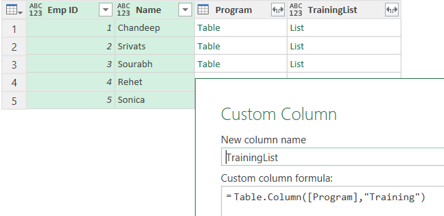
To create a List from the Training Name. Click on Custom Column from the Add Column Tab and write the following Formula

Table.Column([Program],'Training')

Note that Power Query is case sensitive, don’t you dare make any errors 😉

This will generate a new Column with a “List” in each row. Simply Click on Double Headed Arrow Icon in the Header “Training List” and choose Extract Values >> Choose a Delimiter

You’ll see all values have come in a single row, separated by the delimiter. I guess you got now.. all that is left to do is >> Right Click and Separate the column with the same delimiter and you have separate columns for each row. Of course after removing any junk columns our data looks like we wanted.

Each row (for training) has been transposed in to a separate column… nifty huh!!

All you do now is Close and Load 😎

 

In case you understand better with Video.. I got you covered 🙂

 

In case you had to solve the problem, how would you have tacked it ? Let me know in the comments

DOWNLOAD THE SOLUTION EXCEL FILE FROM BELOW

 

More Power Query Cases/Problems

1. VLookup for Duplicate Records (& extract them in a single row)
2. Convert Multiple Columns to Rows
3. Leave Data Analysis using Power Query
4. How to do a Vlookup in Power Query
5. UnPivot Data with 2 Headers
6. Find Unique Dates Challenge
7. Merge Data from Multiple Excel Files using Power Query