Change Measures Using a Slicer in Power BI

One of the most common questions that I get is, how can I change measures using a slicer? In this post I’ll exactly show how can you do that in Power BI.

Want to start with a Video?

Consider this simple data model

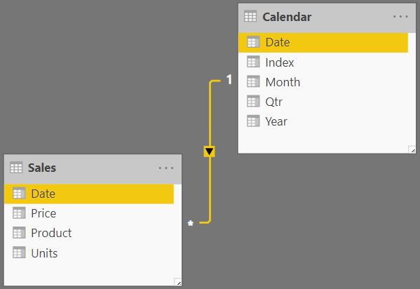
1. We have the Sales table connected to the Calendar (Date Table)
2. The Sales table has standard columns like Date, Price, Product and Number of Units

Using the above model I create the below Pivot Table with 4 Measures – Total Sales, Total Units, Transactions, Unique Selling Days

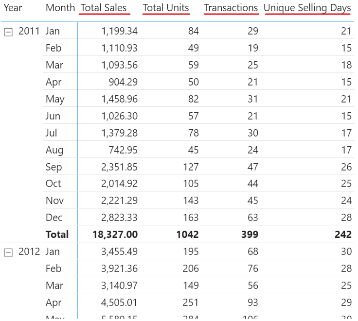
The measures are below!

Total Sales = 
SUMX(
    Sales,
    Sales[Units] * Sales[Price]
)

Total Units = SUM(Sales[Units])

Transactions = COUNTROWS(Sales)

Unique Selling Days = DISTINCTCOUNT(Sales[Date])

Now instead of displaying all the measures in a single Pivot Table, I’d like to choose from a slicer the measure that should appear in the pivot table.

Using a Slicer to Select Measures

Before I go on to explain the way to set this up, I’d like to break down the technique into 3 main steps.

• Step 1 Creating a Slicer – Note that slicers can be created on a column of a table. So we need a table that has a column with 4 values i.e. (Total Sales, Total Units, Transactions and Unique Selling Days)
• Step 2 Capturing the value selected in the Slicer – When the user selects any measure in the slicer, I should be able to capture his selection.
• Step 3 Dynamic Measure based on Slicer – Based on the selection made in the slicer, the measure should change to the calculation selected.

Step 1 – Creating a Slicer

First, I need a table with a single column with 4 values (i.e. names of the measures). Since I prefer DAX, I’ll do the DAX way (it’s easier to edit if I need one more value to be added later).

From the Modelling Tab >> New Table >> Use this code

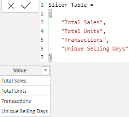
Slicer Table = 
{
    'Total Sales',
    'Total Units',
    'Transactions',
    'Unique Selling Days'
}

I get a nice little table with a single column containing the names of the measures.

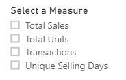
This table won’t have any relationship with any other table (it’s on purpose a disconnected table). Now that I have this table, I can create a slicer on the value column of this table.

Step 2 – Capturing the Value selected in the Slicer

As now nothing happens when the user selects on the slicer. Unless I capture what the user has selected in the slicer, I won’t be able to create dynamic calculation.

To capture what the user is selecting, I create this simple measure

User Selection = SELECTEDVALUE('Slicer Table'[Value])

1. This measure will return whatever the user selects in the slicer.
2. If the user selects nothing or more than one value in the slicer, I get an alternative result as Blank.

See the result.. looks good!

Step 3 – Creating a Dynamic Measure

Now that we have captured what the user has selected, I can write this dynamic measure to toggle between calculations as per slicer selection. See this measure

Calculation = 
SWITCH(
    TRUE(),
    [User Selection] = 'Total Sales', FORMAT([Total Sales],'0,0.00'),
    [User Selection] = 'Total Units', FORMAT([Total Units],'0'),
    [User Selection] = 'Transactions', FORMAT([Transactions],'0'),
    [User Selection] = 'Unique Selling Days', FORMAT([Unique Selling Days],'0'),
    'Select any Single Calculation'
)

Don’t get intimidated, read this measure as a simple nested IF

• IF the user has selected “Total Sales” THEN run [Total Sales] calculation
• ELSE IF the user has selected “Total Units” THEN run [Total Units] calculation
• and so on..
• ELSE if nothing or more than one value is selected show a message ” Select any single Calculation”

The FORMAT function is used to format the style in which the numbers appear. So for instance, I wan’t [Total Sales] to have 2 decimals with commas. Smart isn’t it 😎

Let’s drag this to our Pivot Table and see the result

Works just fine!

One additional anomaly that you’ll face is that the Calculation measure result will be left aligned because we have used the FORMAT function, which converts it to a text value.

You can go the In the Format Pane >> Field Settings for Calculate >> Make it Right Aligned and that problem is fixed

Creating a Dynamic Title

It would unfair to end this post without fixing the bad title “Calculation”. The user must see the actual name of the measure as a column header.

Yeah.. but it’s not doable (or I don’t know a way to do that) but I have a quick fix,

1. I’ll create a multi row card with the measure User Selection (which displays what the user has selected).
2. Format the card – Remove the side bar, adjust size and font, remove the label etc..
3. And place it on top of Calculation
4. Group the two objects and it looks super slick and indistinguishable

take a look..

Guys from PowerPivotPro wrote about the same problem here.

Need more dose of DAX ?

1. Calculate Non Blank Values – Smart Trick
2. Calculate Fiscal Week 
3. Financial Year Calculations in Power BI
4. Slab Based Calculations
5. Sort by Column – Interesting Examples
6. Top Selling Product Analysis – Case Study
7. Least Selling Product Analysis  – Case Study