Change Pivot Table Values Field using VBA

Recently while working on an HR Dashboard I worked out a nifty solution to change the calculations for a pivot table dynamically using a short VBA code.

I am going to do a complete tear down of how did I do it. Let’s take a dive!

 

Consider this Data & a Pivot Table!

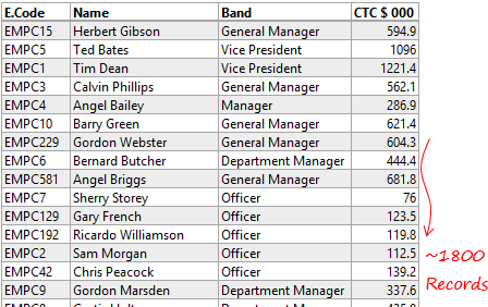
And we create a simple pivot from this data set. Band in Rows and CTC in Values. Nothing sophisticated until yet.

 

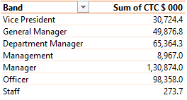
Step #1 – Creating Dummy Calc Table

Next to Pivot Table I have created a small table with the following data

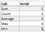
The Calc column depicts the type of calculation and there is a Serial number for each. If at all you are wondering why are the Serial numbers in the right column, Well.. no reason.. just like that! 🙂

 

Step #2 – Creating a Pivot from the Calc Table

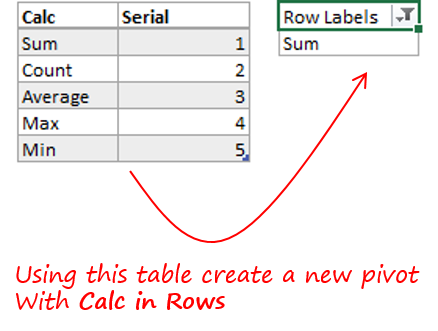
Then insert a Slicer on the Calc Field

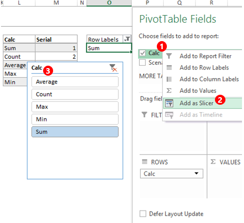
1. In the field list, right click on Calc
2. Choose Add as Slicer
3. Slicer is created!

 

I am assuming that you now understand the purpose of creating the dummy Calc table and the Slicer. If you haven’t, read on..

1. The Calc Table –
   • Is a dummy that will support some further calculations and
   • It can also be expanded to contain more calculations (like Std Deviation, Variance, Distinct Count etc..) other that the ones mentioned
2. Slicer – Is just a dynamic selection tool for the calculation that we want to perform

 

Our next task is to connect the slicer with the Pivot Table calculations.

 

Step #3 – 2 More Dummy Calculations..

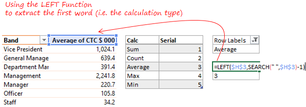
The LEFT & SEARCH are used to extract the first word from our first Pivot Table. This will tell us what calculation is currently performed in the Pivot Table

Next Calculation is a quick VLOOKUP to find the serial number

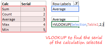
Note that our slicer is connected to the pivot table, so when we change the Slicer selection the row labels update and the Vlookup value (serial no) also updates

Finally name the cells..

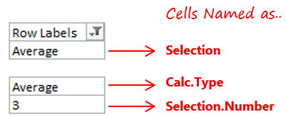
Cell naming is important because we will refer to these cells in our VBA Code not with their cell addresses but by their names. This makes the code a bit more robust

Learn Cell Naming in detail

 

Step # 4 – Time for some VB coding..

Here is the sweet little piece of code that ties everything together. Feel free to customize by changing the text in blue

Private Sub Worksheet_Change(ByVal Target As Range)
 If Not Intersect(Target, Range("Selection")) Is Nothing Then
Dim Pvt As PivotTable
Dim Pf As PivotField
Dim Sh As Worksheet
Set Sh = ActiveSheet
Set Pvt = Sh.PivotTables("PivotTable1")
 
If Range("Selection") = Range("Calc.Type") Then
 Exit Sub
Else
For Each Pf In Pvt.DataFields
 Select Case Range("Selection.number")
 Case 1
 Pf.Function = xlSum
 Case 2
 Pf.Function = xlCount
 Case 3
 Pf.Function = xlAverage
 Case 4
 Pf.Function = xlMax
 Case 5
 Pf.Function = xlMin
End Select
Next Pf
End If

 End If
End Sub

 

To use this code..

1. Copy it from above
2. Use ALT F11 to open the VBA Window
3. In the Workbook
4. Double click on Sheet 1 (or whichever sheet you are working on)
5. And paste the code there!
6. Close the VBA Window 🙂

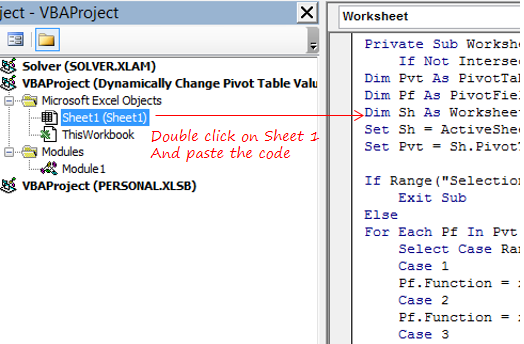
Don’t forget to save the file in xlsm format.

 

Now when you play with the Slicer the Pivot auto updates!

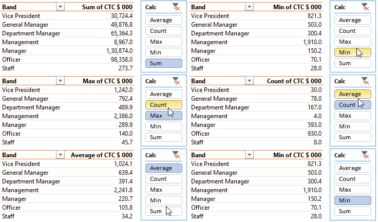
I like to format my Slicers.. so when you download the file, you’ll see mine a little more fancier than yours. But feel free to copy mine if you wish to 😀

 

DOWNLOAD THE EXCEL FILE

 

For Video Lovers!

 

If you struggle to apply this trick to your own data, please don’t hesitate to leave a comment. Also where all do you think you can apply this in your work.

I would love to hear from you

 

More Pivot Table Tricks!

1. 16 Time Saving Pivot Table hacks
2. Boost the power of your Pivot Table by using Data Models
3. Pivot Table Data Ranking Trick
4. Unpivot the Data using Pivot Tables