If you and I interact on emails, you know that I asked you this question. Nevertheless even if you are a first timer, let me start from the top and explain you the case
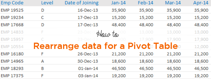
Take a look at the data below.
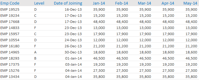
Nothing much to explain, we have a matrix with
- Employee Code
- Level
- Joining Date
- And against each employee code we have 24 months of Salary (depending on joining date)
So, if I asked you a question – Tell me the Level wise, salary payout quarter by quarter in the year 2014 and 2015? How would you solve this question
If you are an avid pivot table user you’ll notice 2 things
- You can solve this under 30 Seconds
- But the problem is that this data is not kept in way, which can be used in a pivot table
So whats wrong with this data?
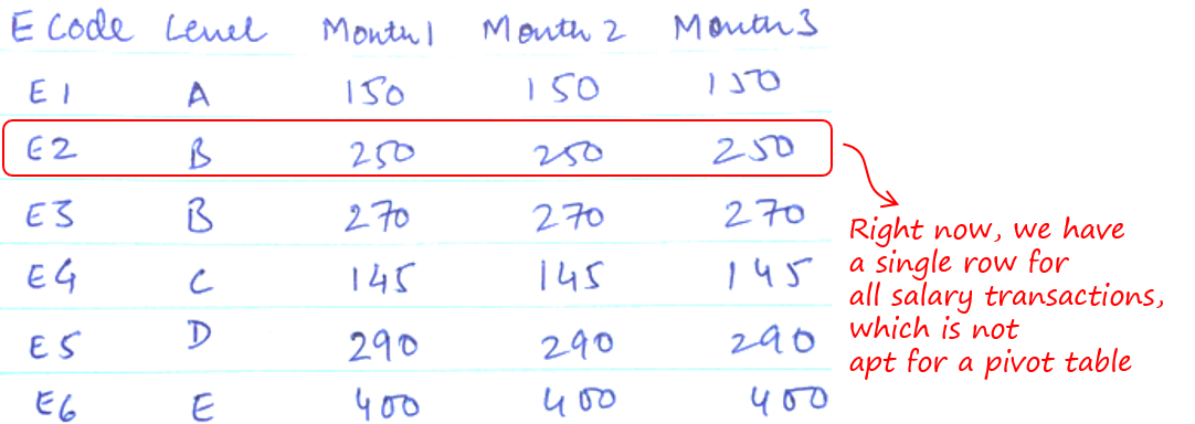
Each employee is occupying a single row for showing salaries for all the months. Where as each salary should be a single transaction and should be displayed in a single row
This is how the ideal data should look like
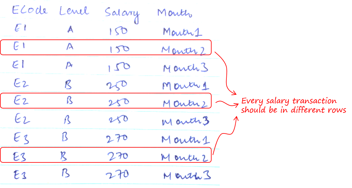
So our first task will be to re-arrange this data, even before we approach pivot tables!
Transforming the Structure of the Data
Had it been a few employees, one could have still managed to do some manual work. But now that we have 500 hundred employees, we really need to think out of the box!
At-least I am not the one reorganizing 12,000 rows of data (500 employees x 24 months) manually. So let’s begin with some smart ass tricks!
1) Create a Pivot Table, but not the usual way
- The default way to create a pivot table is to click to on Pivot Table from the Insert Tab, but that is not our way for this case
- Let’s invoke the old pivot table wizard using the Excel 2003 shortcut: ALT D P. Pivot Table wizard will open up
- Select the option Multiple Consolidation Ranges
- Next select the option Create a single Page field for me
- And then pick up the entire range of data and click on the Add
- Insert the Pivot Table on the New Sheet
Once you get the Pivot Table
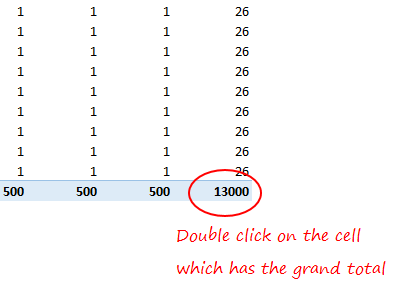
- Double click on the last cell which displays the grand total
- Double clicking on that cell will expand the summarize data in the manner that we want. You’ll get something like this (look at the picture below)
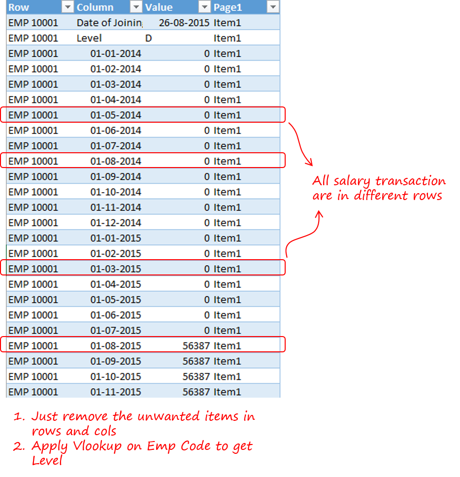
Now that we have the data the way that we wanted. We need to do 3 more things
- Remove the extra column that is created – Page1 is not useful to us
- Apply filter on column B and remove row items which contain the text Date of Joining and Level.
- Apply Vlookup on Employee Code and get the Level of the employee form the main data
3. Finally Create a Pivot Table with the new Data Set
- Create a Pivot Table
- Drop Levels in Rows, Salary Dates in Columns and Salary in Values
- Now group the dates by Month and Year
- Done!
More Pivot Table Resources for You
- A Comprehensive Pivot Table Course and Sales Dashboard – I released it on my birthday last year and it is free!
- Introducing Calculated Columns in Pivot Tables
- Grouping Feature in Pivot Tables
- Put your Pivot Tables on Steroids with Data Models – Excel 2013 feature