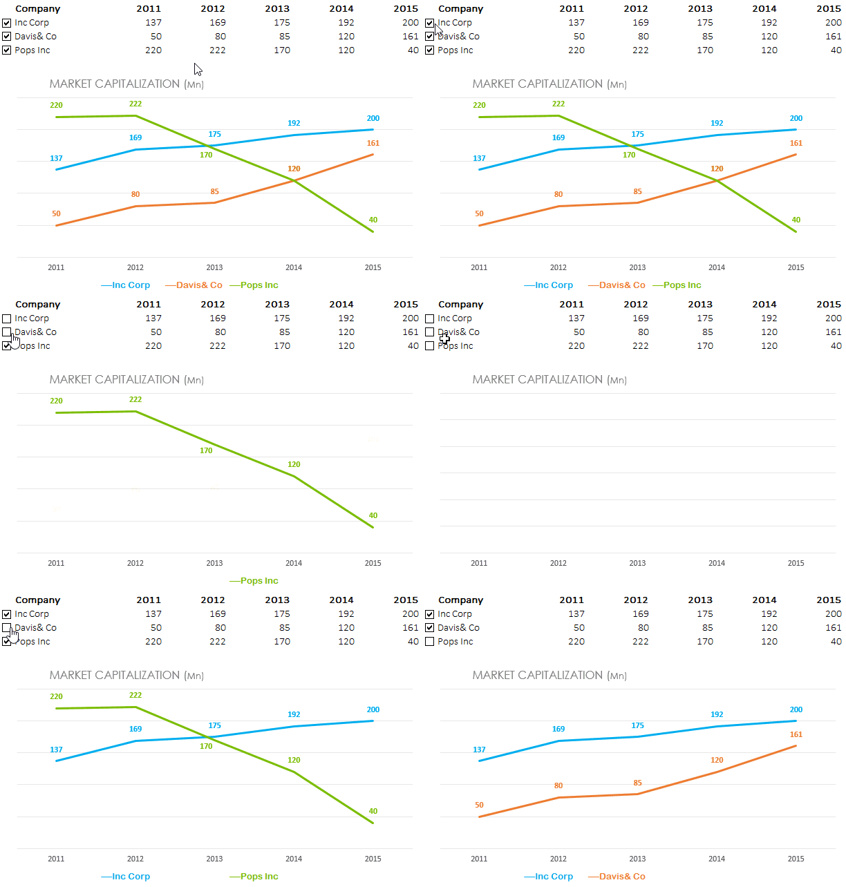
I guess I don’t have to say much to get your interest!! Interested..? Ok lets begin! 🙂
Here is our data

Three companies with Market Capitalization (in simple words the worth of the company) figures for 5 years. Apart from the data we need 3 more things
- A Line Chart – Which is not too difficult 😉
- The Check Boxes – We’ll create these in a moment
- A technique to connect the Check Boxes to the Chart
Creating Check Boxes
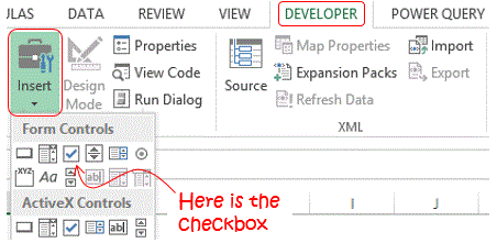
- For creating the Check Boxes you first need to Activate the Developer Tab
- In the Insert drop down you will find the Check Box. Make sure to choose the one under Form Controls and not the one under Active X Controls (I’ll talk about “WHY” sometime later)
- The mouse cursor will turn like a + plus sign. Simply drag to draw a check box
- And then create 2 more copies of the Check Box. One for each company
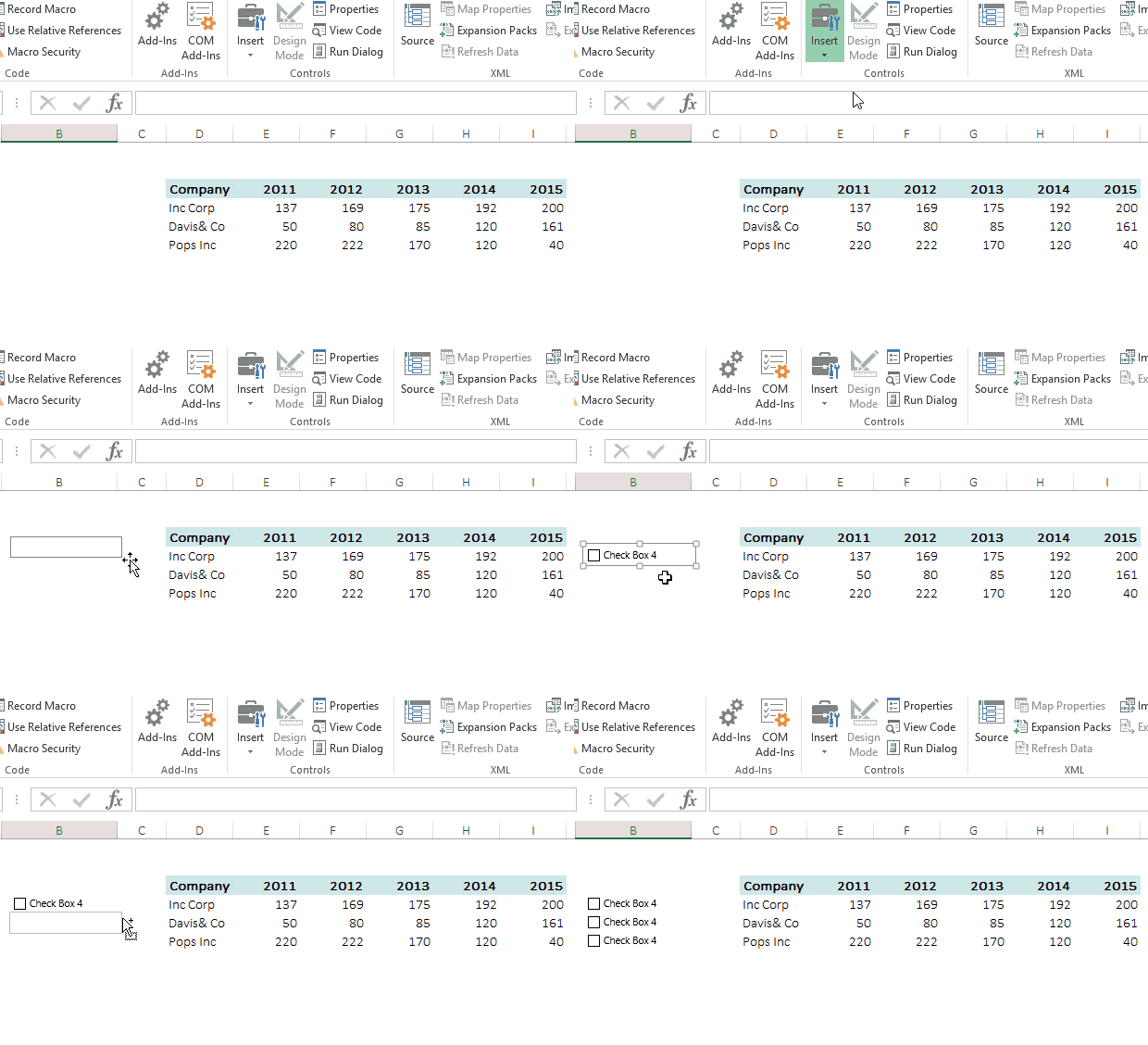
Quick Tip: To select the check box hold the CTRL key and then click on the check box
Linking the Check Boxes to the Spreadsheet
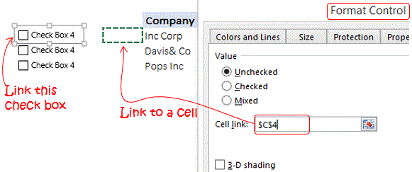
- Select the Check Box (using CTRL key) and in the right click menu go to Format Control
- Link the cell link to a cell address (preferably next to the company name)
- Do the same for all the Check Boxes
- Now when you click the check box the linked cell shows TRUE (checked) or FALSE (unchecked)
Now we need to link the linked cells to our data for which let’s prepare a quick dummy
Preparing Dummy Data for the Chart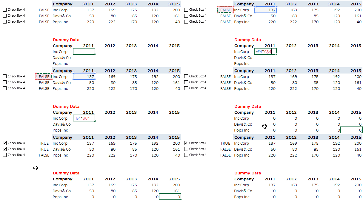
The Logic : Just like computers Excel understands TRUE as 1 and FALSE as 0
- To prepare the dummy data, we are multiplying the TRUE & FALSE (in the linked cells) to the actual values
- So when we un-check the button, the dummy values becomes 0 (i.e. number x false)
- And when the button is checked, the dummy value appears ( i.e. number x true)
Creating a Chart with the Dummy Data
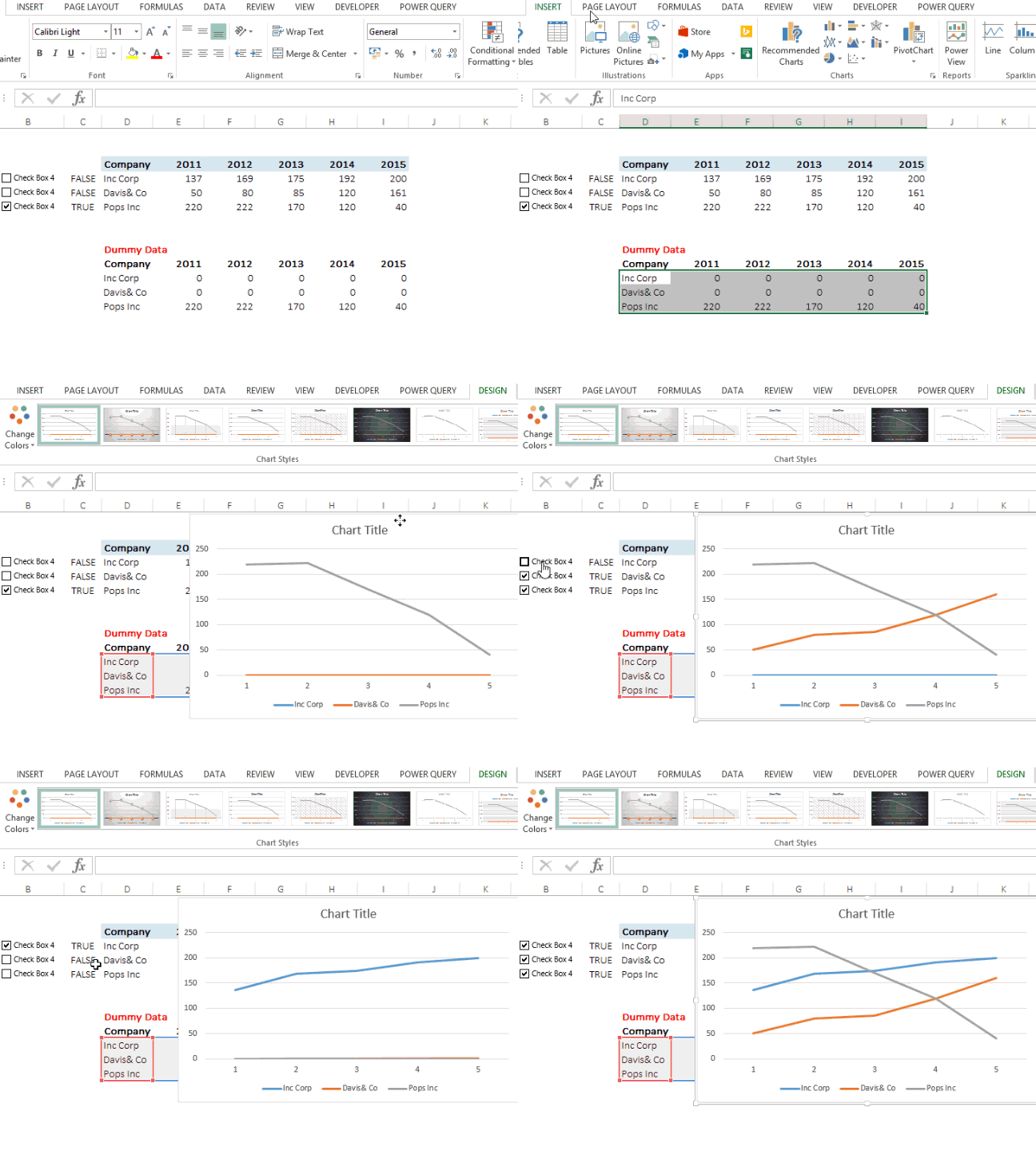
- Select the data (companies & values) and make a line chart
- Click on the Check Box to pick the company you want in the Chart
- All you need to do is a bit of formatting to the chart to make it look sexier! [Read Chart Basics 1, Chart Basic 2 & Chart Basics 3]
