The Offset Function & Applications

The Offset function is one of the big daddies of the Lookup functions family and brings new possibilities in Excel but is if often suggested to use with caution because of its volatile nature. Lets cover the Offset and its applications in depth!

 

Just for understanding purpose let’s divide the Offset syntax into 2 parts (the basic and advanced)

Offset Syntax (Basic)

The basic offset syntax has 3 arguments

 

 

1. Reference – This is starting point (cell address like A1, A10, B5 etc..) from where you want to start your lookup
2. Rows – The number of rows you want to move up (-ve number like -4, -2 etc…) or down (+ve number like 2, 3 etc..) from the starting point (Reference)
3. Cols – The number of columns you want to move left (-ve number like -4, -2 etc…) or right (+ve number like 2, 3 etc..) from the starting point (Reference)

 

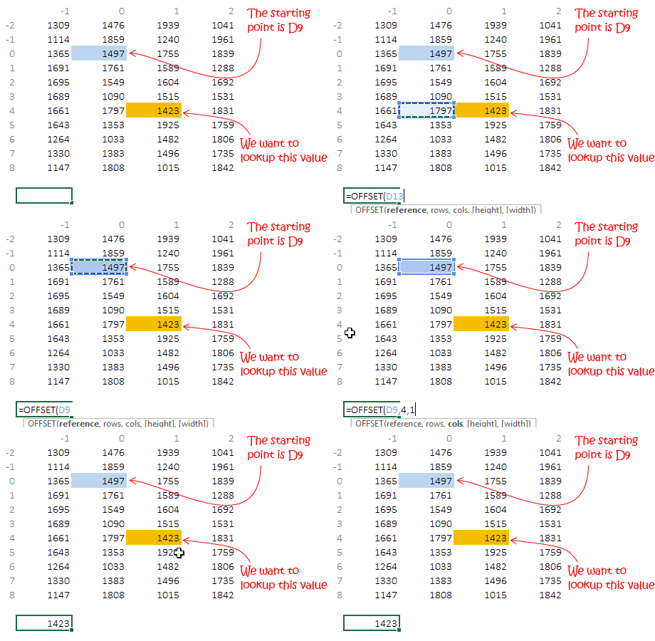
Let’s look at a case

 

 

 

 

 

 

 

 

A few things to note

1. Reference: We start at D9 so that cell (for offset) becomes the 0th row and 0th column
2. Rows : We enter the value 4, so the offset will move down 4 rows
3. Columns : We enter the value 1 so the offset will shift one column to the right and gives the output as 1423 (which is 4 rows downs and 1 column to the right of the reference)

Remember: In case of  Vlookup or Index functions you specify an array and the first column of that array is marked as 1 but in Offset the starting point (Reference) is marked as 0th row and 0th column and then depending on your input in rows (+ve or -ve) and cols (+ve or -ve) you can move anywhere on the spreadsheet

 

Offset Syntax (Advanced)

Two more options get added here : Height and Width (both are optional). These options help you form dynamic arrays..eh?? confused ?? 🙄 Let’s check them out

4. Height – How tall should be your array(i.e how many rows vertically?). The height can be +ve (downwards) or -ve (upwards)

5. Width – The wide should be your array (i.e. how many columns horizontally?) The number of columns can be +ve (rightwards) or -ve (leftwards)

 

The same case once again

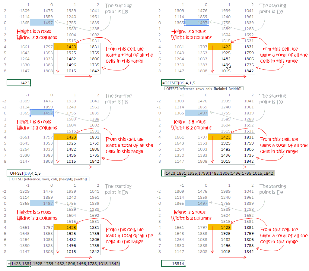
1. We are just entering the height as 5.
2. And Width as 2.
   • It allows the offset formula create a 5 x 2 matrix starting from cell value 1423
3. Since the (stand alone) Offset formula is not specified to do anything with the matrix, it gives a #VALUE! error
4. So we just wrap the Offset around the SUM function (or any other function like MAX, MIN, AVERAGE or even use the Matrix in the INDEX function)

 

Now it could be hard to imagine the application of Offset but it can help you achieve the impossible. I have 2 quick real time application for you

Application of Offset I – (Financial Modeling)

Here we have new assets being added in different years and we have to apply a Straight Line Depreciation Method (Fixed Depreciation i.e. Asset/Life) each year. Here is how we can use Offset

1. Since our assets are completely depleted every 3 years we only want to total the last 3 year assets
2. We use Offset
   1. Reference or Starting Point – E20 (Current Year)
   2. Rows – We don’t want to move any rows
   3. Cols – We don’t want to move any columns
   4. Height – We don’t want any rows as height
   5. Width – Here we specify -3. WHY? because we want to make an array of last 3 year of assets and add them, so wrap our Offset in the SUM function
3. Now just divide the asset balance by 3 (asset life) and you get the depreciation

This is one of the easy ways of doing it!

 

Application of Offset II – (Dynamic Charts)

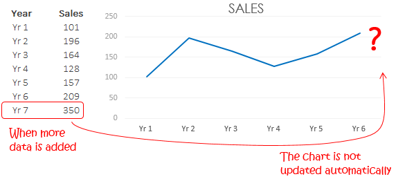
Here is what we do

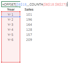
We create dynamic ranges using Offset for years

1. Reference – We starting counting the data (filled cells) from $B$18 (lock it)
2. Rows – No rows
3. Cols – No columns
4. Height – We want to have all the filled cells in the a range for which we use =COUNTA(On a range little larger than our data). This is going to give the count of the filled cells (in our case 6)
5. Width – No width

The Offset will create an array of 6 numbers. When you press enter the Offset will give a #VALUE! error (since it cannot display six numbers in a cell) but that is okay

We similarly create a range for Sales

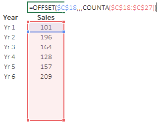 --> The Offset will create an array of 6 sales figues

Now create two dynamic named ranges using cell naming

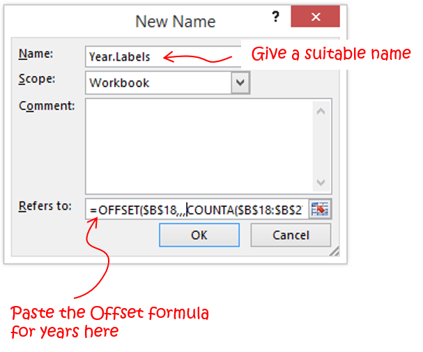
1. Just click on Define Name in the formulas tab
2. Paste your formula in the Refers to region and (make sure to have all the cells locked)
3. Give a suitable Name

Repeat this process for the Sales range as well.

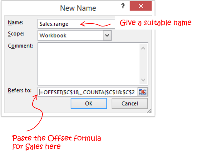
Now we have 2 named ranges. You can choose to delete the 2 offset formulas that we created on top of data

Now link the named ranges to the chart. Read more on how to do add data to chart, chart formatting & charting options in Charts Part 1, Part 2, Part 3

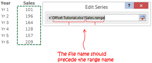
Similarly link the years on the horizontal axis labels

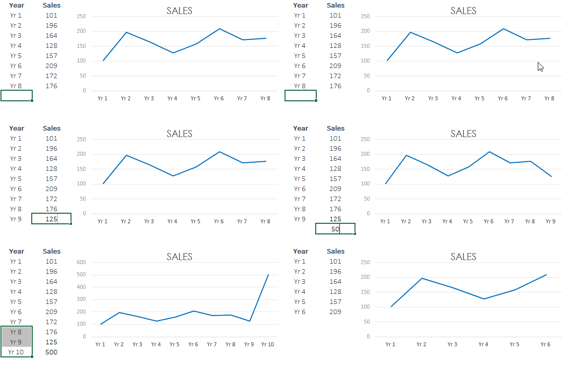
Now when you add more add more (or delete) data, your chart will automatically update.. thanks to Offset!!

 

Offset Function and its Volatile Nature

The Offset function would recalculate itself each time Excel recalculates. In simple words it keeps your Excel busy by running the offset formula over and over again, which can be quite dangerous if you are working with heavy data or financial models. If you wish to read more about volatility or volatile formulas like Offset you can visit Charles Willams’s article on Volatility or read a new year (2010) resolution from Dick Kusleika – no more Offset

 

Do you use Offset?

How often do you use Offset? or do you keep your self from using it? Please share your views using comments