Unpivot Data with 2 Headers

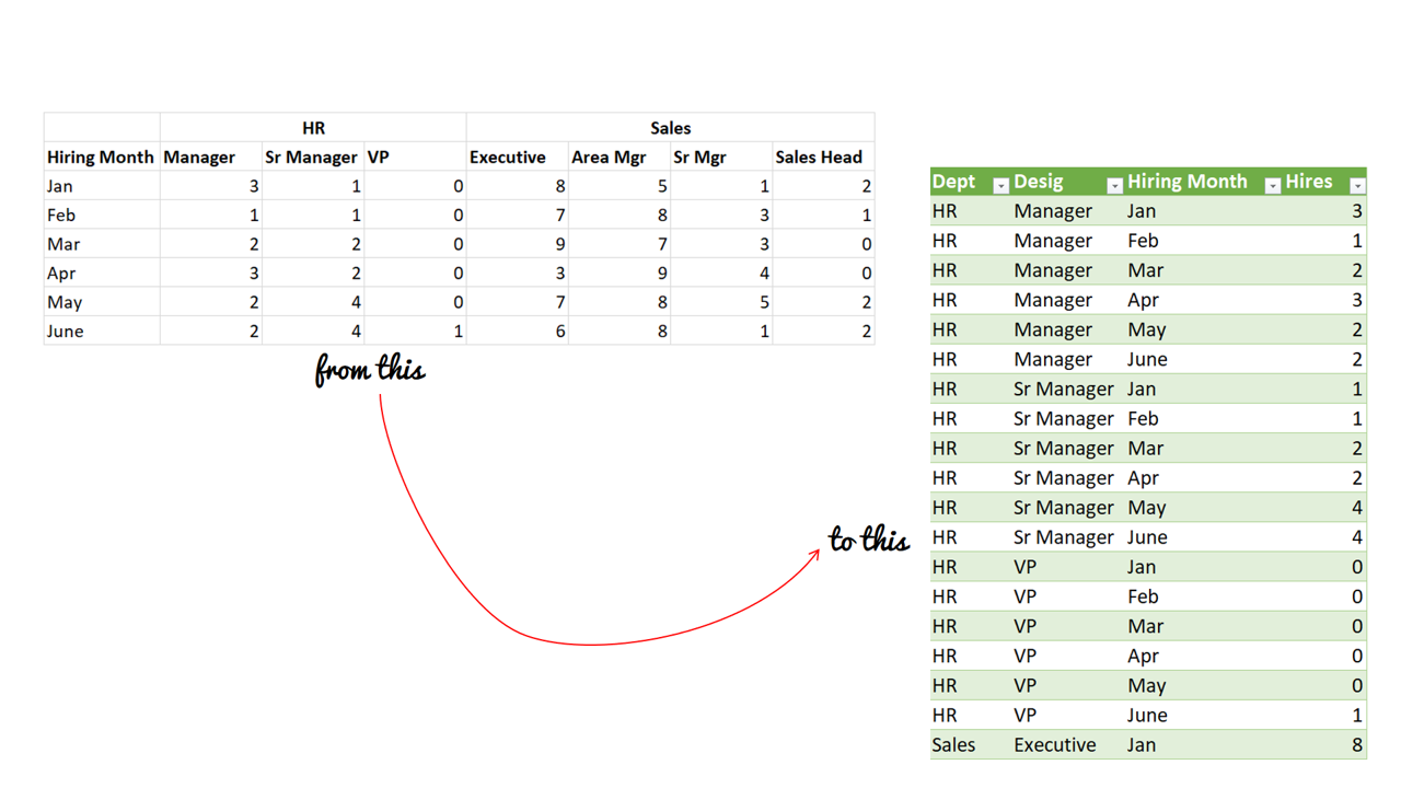
Imagine this tiny data set!

Couple of problems with this

1. If you tried to make a pivot from this data, it would simply deny since you have merged column headers on the top
2. The other challenge you’ll face is that this data is not Pivot Table ready
3. You’ll need to have a separate row for each number with 3 separate columns for Department, Designation and Hiring Month.

 

This is a common problem people face with they have data with 2 headers. Let’s solve this! Enters Power Query

 

Load the Data in Power Query

I named the range of data as “Data” and loaded it in Power Query. It shows up something like this

 

Next let’s transpose the Data. From the Transform tab > Transpose

I guess you got the sense that un-pivoting this now is easy but before that let’s massage our first column (Dept) a bit

 

Select the Column1 and click on Fill>Down from the Transform Tab. This will fill up the nulls and Promote the first row to Headers (from Home Tab). Our query now looks something like this

 

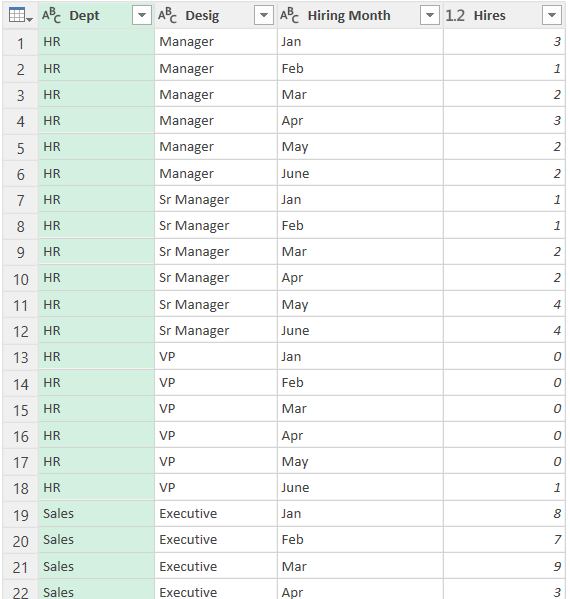
This is the step that you have been waiting for. Select the first 2 columns > Right Click > Unpivot Other Columns. Also suitably rename the columns and boom you are done!

 

Video Lover? Watch this

 

 

Some more interesting Power Query Tutorials

1. Repeat Row N Times
2. Vlookup in Power Query
3. Leave Data Analysis in Power Query
4. Combine Duplicate Vlookup Values in a Single Row
5. Merge Data from Multiple Excel Files