Use Camera Tool to make Dynamic Charts in Excel

Excel has some pretty kick ass unique features and one of them is the Camera Tool. On the face of it, it looks like no big deal. But the camera tool when combined with a formula and options buttons, can help you make a pretty awesome dynamic chart

Let’s get right into it!

 

So let’s say we have this data..

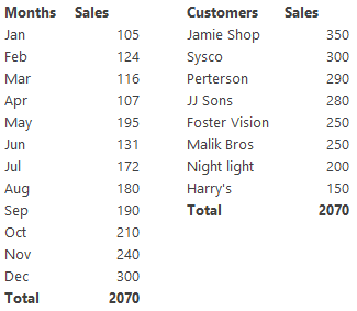
Revenue Split by Months and Customers

 

And we have made 2 charts from the above data

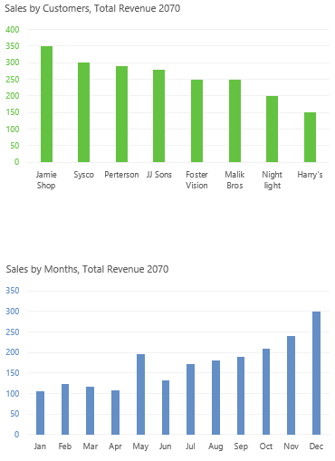
Our objective is to show one chart at a time (either Sales by Months or by Customer)

 

Now Let’s Create the Option Buttons..

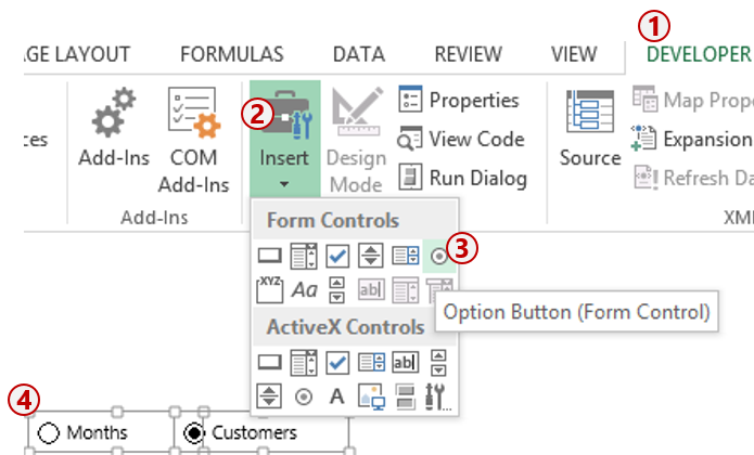
1. From the Developer Tab [Related: Activate the Developer Tab in Excel]
2. Go to the Insert Drop Down
3. And Click on Option Button (Form Control)
4. Using the cursor draw 2 Option Buttons and rename them as “Months” and “Customers”

 

Connect the Option Buttons to a cell

1. Name a cell (above your option buttons) as “Choice”
2. Right click on the Option Button and go to Format Control
3. In the Cell Link : Type the name of the cell “Choice”
4. Now when you click on the Option Buttons the named cell will indicate 1 or 2 (depending on the option button selected)

 

Let write a Choose formula for picking up the chart range..

[Related: Learn how the Choose formula works]

Note that :

1. The ranges selected in the Choose Formula are completely covering the cells where the chart is kept.
2. So you need to arrange your charts in such a manner that they fit in a range of cells
3. The ranges are also locked ($ sign). If you don’t do that we would have problems while naming the formula later
4. Don’t worry about the #VALUE! error

 

Now name this Formula as Pic.Choice

1. Copy the Choose Formula that we have just created
2. Open the Name Manager (Ctrl + F3)
3. Create a New Name – Pic.Choice
4. Paste the choose formula in the Refers to box

 

Time to use the Camera Tool..

1. Select the range covering any of the charts
2. Then click on the camera [Related: activate the camera tool]
3. Now when you click anywhere on the spreadsheet the picture of selected cells will be pasted

 

Final Step : Link the Picture to the Choose Formula

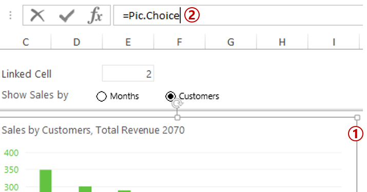
1. Select the Picture clicked by the camera tool
2. Go to the formula box and link it to the choose formula =Pic.choice
3. Make sure to press enter after you type the name of the formula
4. Done!

 

Caution: If you reposition the charts on the sheet. The range that you have selected the choose formula will no more be captured the chart

How does the Chart work..

If you have found this a bit tricky, let me help you to get your head around this

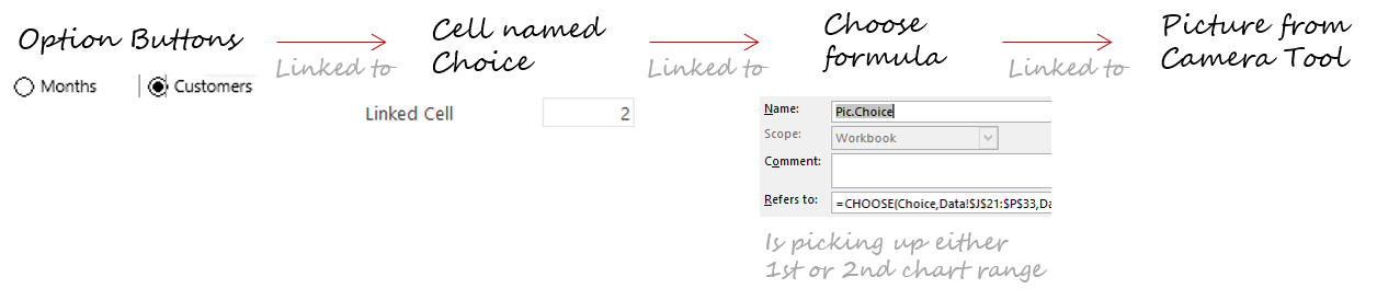
1. The picture from the camera tool was linked to the range covering the chart (which was selected manually)
2. But when you link the picture to the choose formula the picture becomes dynamic and gets connected with the option buttons
3. So when you change the option buttons the range selected also changes, so does the chart!

 

Other Interesting Chart Types

1. Learn how to work with Camera Tool from Scratch
2. Do a Picture Vlookup in Excel
3. Threshold Chart in Excel
4. Check button Chart
5. Make a Chart with a REPT Formula