Find the Top ‘x’ Items [Pivot Table Trick]

When you make a pivot table not necessarily we need the summary of all the items, there have been instances where I needed only Top 5 or Top 3 items to be displayed in the pivot table.

Here is a little trick that can help you do it with a few clicks

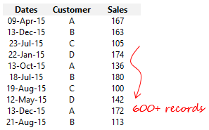
Let’s say we have this data

and we created a pivot table from this data

1. Where the dates are grouped in quarters and are in Columns
2. Customer dropped in Rows
3. Sales in Values

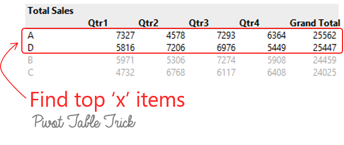
Now what if I wanted to only see top 2 Customers (by total sales) in the Pivot Table ?

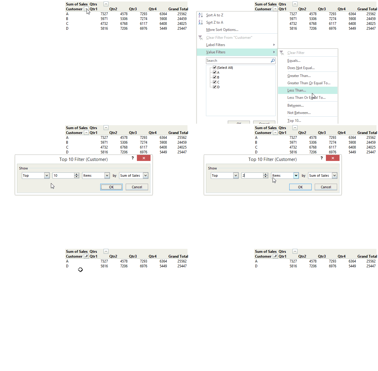
1. Click on the Customer Filter in the Pivot Table
2. And go to Value Filters and further select Top 10
3. In the option box select Top 2 items and
4. Click on Ok

The records get filtered only to the top 2 items. You can similarly customize it to top ‘x’ items

The cool thing is

1. Just as the way I have filtered the Customers in Rows, you can also filter the Quarters (or anything else) in the rows
2. If the source data changes, pivot table filters also get refreshed when the pivot table is refreshed

More Pivot Table Tricks

1. 16 Life and Time saving Pivot Table Tricks
2. Unpivot data using Pivot Table
3. Calculated Fields in Pivot Tables
4. Data Models in Pivot Tables