16 Life and Time saving Pivot Table Tricks

Today let me share with you 16 gold nuggets that will help you save your time while crunching numbers with pivot tables! Excel hacks are equivalent to gold nuggets for people like us.. aren’t they? Lets get started

 

1 Use Tables Instead of Normal Cell Ranges

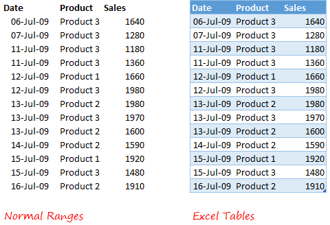
Before creating a Pivot Table convert your data into a Table

1. Simply click on any cell inside your data range
2. Use the Shortcut Ctrl + T (make sure that your table has got headers)
3. Click on OK. Done!

Benefit of using a Table – Tables have self expanding feature, so when more data gets added, you won’t have to change the source data in the pivot table. [Related: Take a look at how Tables work in VLookup]

 

2 Get Unique Values

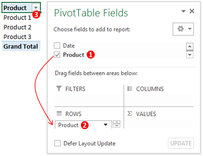
Let say I want to know how many unique products do we have. Just create a pivot table

• Drag the products into rows
• And you’ll have unique products displayed in the pivot table

Read other methods of finding unique values

 

3 Group Dates into Quarters, Months or in any other combination

If you want to see your sales (or any other metric) to be grouped by quarters or months or even in multiple combinations. Then use the grouping feature

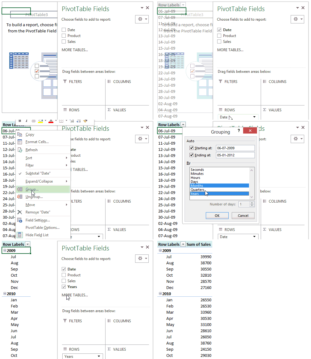
1. Drop the dates in Rows or Columns
2. Click on any date and select Group
3. Pick your choice and the dates will be grouped

 

• Read a more detailed article on Grouping Dates with some other variations
• Read how to create Class Intervals using the Grouping feature

 

4 Rearrange Items in Rows or Columns

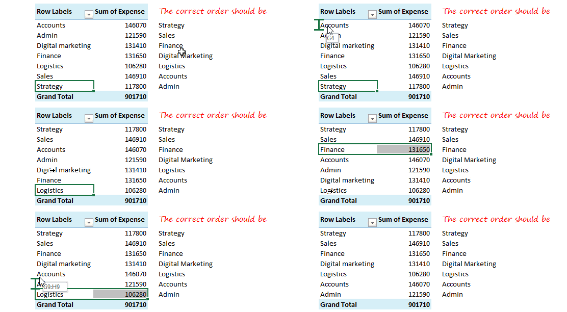
Sometimes the order in which you want the items could more specific. To rearrange items in rows or columns

1. Hover on the item until the icon changes to a Move Icon (with 4 sided arrows)
2. Drag the item to re-position it in the Pivot Table
3. It can be replicated to columns as well

 

5 Do not change the formatting of the Pivot Table Cells

Most often people change the formatting of the cell to get the numbers into a particular format. DO NOT DO THIS

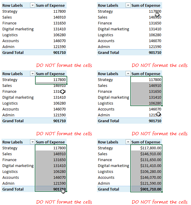
Rather DO THIS

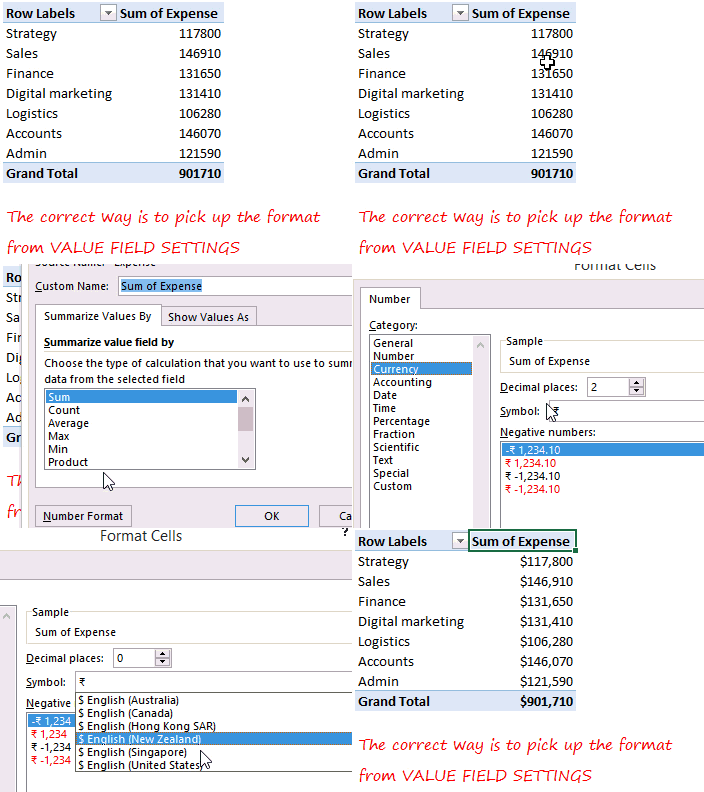
Change the formatting of the field by

1. Right clicking on the field
2. And choosing Value Field Settings
3. Click on Number Format
4. And set the format as per your need

The benefit of doing this: 

1. Excel changes the formatting of the field in the pivot table and not the cell
2. You don’t have to change the format of the cell in case you change the fields in the Value

In short it saves a hell lot of time!

 

6 Drill Down to find the Back up Data

Every once in a while you have the need to find out the back up data behind the value. Let’s say for example I want to see all the values behind January 2010

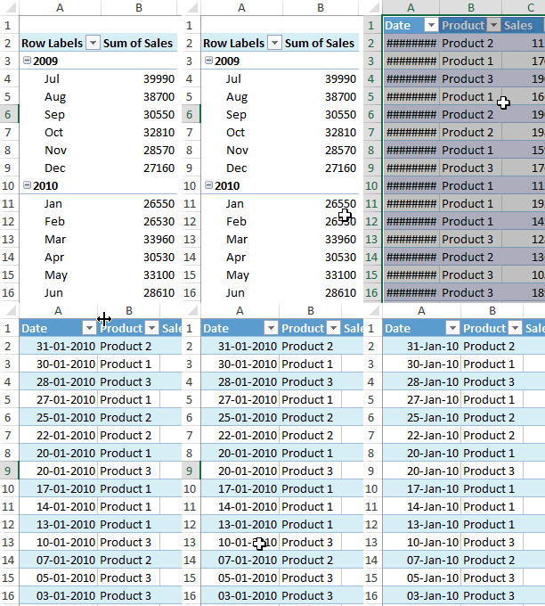
All you have got to do is

1. Double click on the value of Jan 2010 in the Pivot Table
2. Excel will insert a new sheet and show you all the values that sum up the sales of Jan 2010

 

7 The shortcut to refresh Pivot Tables

Shortcut frenzy people can use ALT + F5 to refresh the active pivot table. Please note

1. Your active cell needs to be inside the Pivot Table to refresh it
2. You can use CTRL + ALT + F5 to refresh all pivot tables. The active cell can be in any Pivot Table

 

8 Use Tabular Form to separate the data in different columns

Take a look at the picture below. Right now the products are indented under the departments but what if you want the products in a different column?

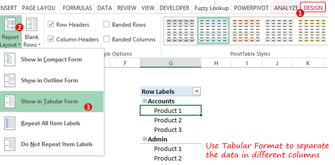
Select the Pivot Table

1. Click on Design Tab
2. In the Report Layout drop down
3. Choose Show in Tabular Form
4. The data will be adjusted in a tabular form

 

 

9 Repeat Item Labels

At times you have the need to repeat the item labels

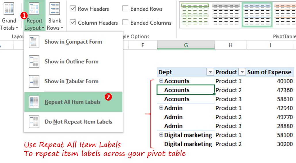
In the Design Tab

1. Click on Report Layout
2. And Choose Repeat Item Labels

 

10 Turnoff GETPIVOTDATA

You might find it difficult writing formulas on pivot tables, because when you do that it refers the cell with =GETPIVOTDATA. Here is how you can turn that off

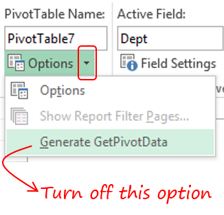
1. Go to the Analyse Tab (Excel 2013) or Options Tab (Excel 2007 or 2010)
2. On the extreme left you’ll see Options
3. Click on the little drop down arrow
4. And check off Generate GETPIVOTDATA

Now your cells in the pivot table will follow the normal referencing style of Excel

 

11 Do Not Autofit Columns

This one is personally very annoying for me when the columns widths are auto adjusted. Here is how you can turn off the annoyance

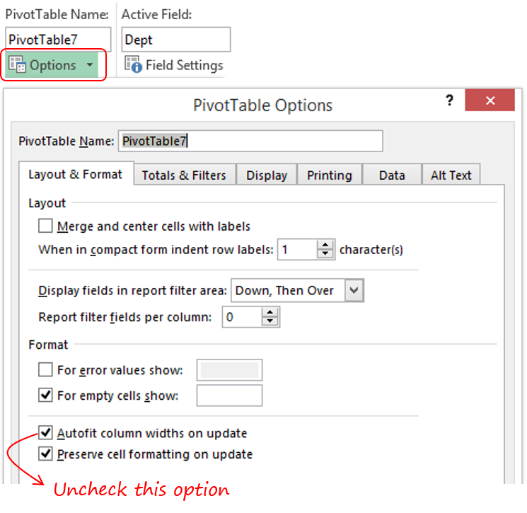
1. Go to the Analyse Tab (Excel 2013) or Options Tab (Excel 2007 or 2010)
2. On the extreme left you’ll see Options
3. In the Pivot Table Options Box under Layout and Format
4. Un-check the Autofit Column Width Option

 

12 Turn off Subtotals and Grand Totals

Sometimes the Sub Totals or the Grand Totals are not needed. Here is how you can turn them off

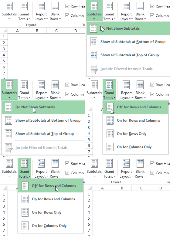
Go to the Design Tab, On the extreme left you’ll find the options for

1. Subtotals – Do not show subtotals
2. Grand Totals – Off for Rows and Columns

 

13 Turn off the Buttons from Pivot Chart

Often people shy away from making a pivot chart because it comes with filter buttons. If you dislike them, here is how you can turn them off

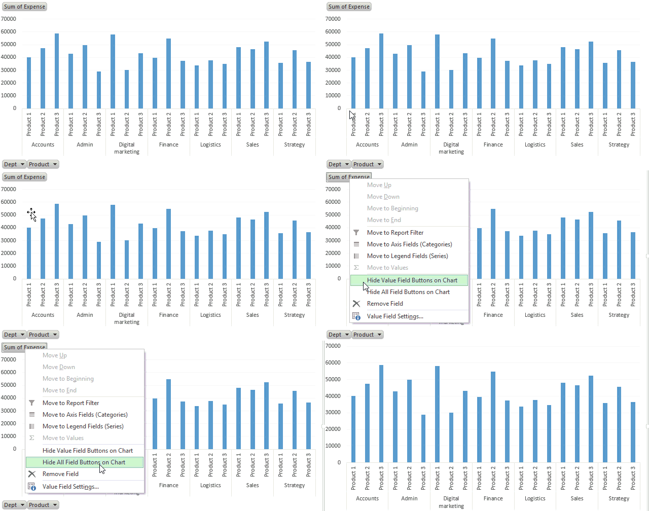
1. Right Click on the buttons
2. And Choose Hide all Field Buttons

 

14 Fill Empty Cells in a Pivot Table

Every once in a while we get empty cells in the pivot table report. If you want to replace the empty cells with something else, here is how you can do it

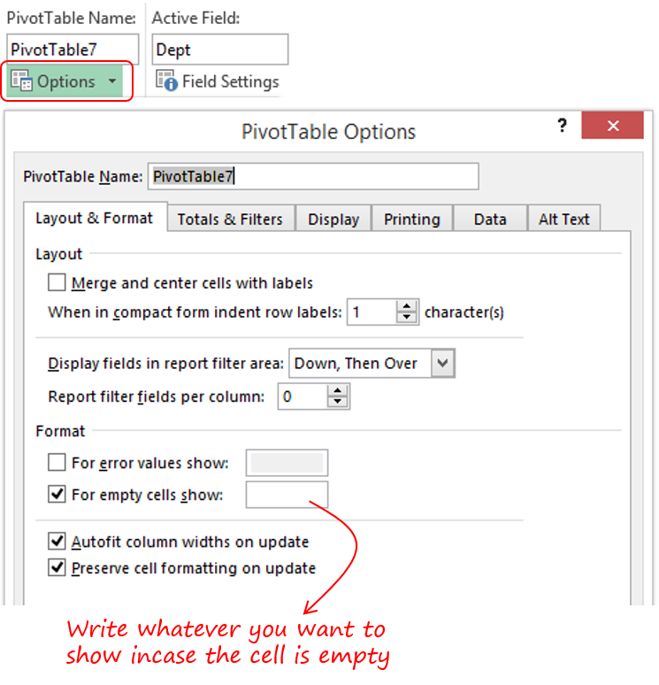
1. Go to the Analyse Tab (Excel 2013) or Options Tab (Excel 2007 or 2010)
2. On the extreme left click on Options.
3. In the Pivot Table Options Box under Layout and Format
4. For Empty Cells Show – Write your value/text that you want to show when the cells are empty

 

15 Delete the Source Data and the Pivot Table still works fine

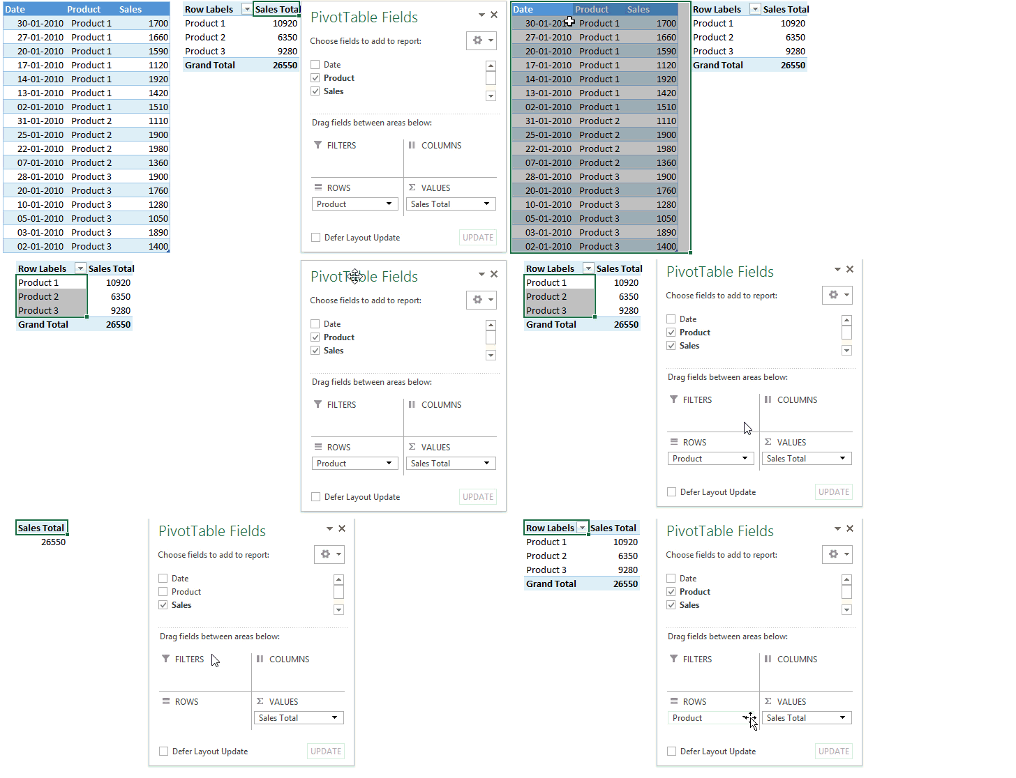
When you create the pivot table the first time

1. It loads the data inside a Pivot Cache (something like the backend of the pivot table).
2. Even if you delete the source data the pivot table is not affected because the data is still stored in the Pivot Cache
3. And it works fine

Things that you’ll be able to do even if you delete the data

1. You’ll be able to work with the pivot table perfectly
2. You’ll be able to drill down and get the data once again when you double click on any pivot table cell
3. Reduce the file size since the data will be only stored in the Pivot Cache

But you won’t be able to – Refresh the data if the source data changes

 

16 Link Multiple Data Sources into a Single Pivot Table

You can link multiple data sources into a single pivot table, rather than first consolidating the data using VLOOKUP. I wrote a detailed post on how can you do that using DATA MODELS in excel 2013 (along with its features). Check it out, you’ll be amazed at what data models can do

 

More Pivot Table Resources

1. How to rearrange the data for a Pivot Table – A must read trick
2. Add Calculated Fields inside a Pivot Table
3. Take a free Pivot Table and Sales Dashboard Course

 

What are your favourite pivot table tricks and which trick did you find most helpful, share them in the comments below!