Use Slicers as Selection Buttons

This is a Chart-Pro’s tip!

If you have been tired of using drop downs or selection buttons (form-x/active-x controls) in your dashboard/charts then it is time that you learn something really cool and fancy

You can instead use Slicers as Selection Buttons!

 

If you already know about slicers then you must be aware that slicers are applied in a pivot table or a normal table which can slice or dice the data

But you can also use them without making a “real” pivot table… well almost! I can’t explain any better if I don’t show you an example.. so let’s get right into it

 

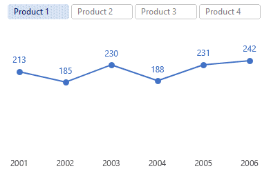
Assume this Scenario

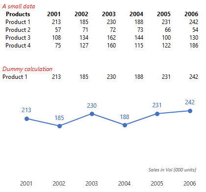
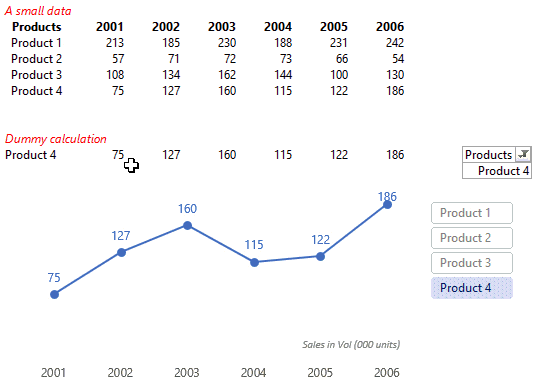
• On the top we have a small data – product volume sales for 6 years
• As a dummy calculation – We have one selected product (via a drop down) and its sales
• And then a chart which shows the sales for the selected product

 

The Problem is – that unless you explicitly mention it somewhere, no user will self get to know that there is a products drop down placed to change between the products

Solution – Well if you are not a formatting freak.. this problem won’t even move the needle for you. I am, and I know a lot of people who are formatting geeks and keeping in mind that you’ll be one of us someday.

I propose to replace the drop down with a slicer for selecting the product. Why? Because slicers are more intuitive and classy

 

To do that

First Create a Dummy Pivot..

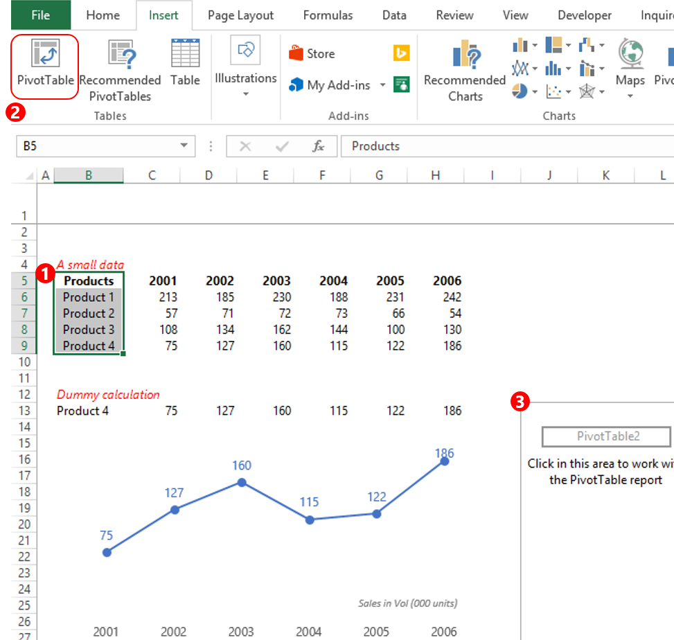
1. Select only the Products column (including the headers)
2. Create a Pivot from the Insert Tab
3. Place the Pivot Table on the same sheet

 

In the Pivot..

You’ll just have one field because we just selected a single column.. which is exactly what we want

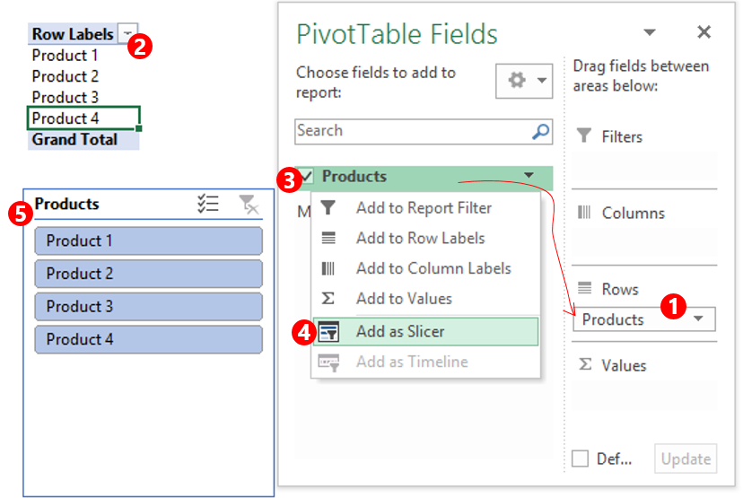
1. Drop the Products in rows
2. You’ll see all products appearing in the Pivot Table
3. Right click on Products in the Pivot
4. And then choose Add as Slicer
5. You’ll get a slicer

Now when you click on the slicer.. you’ll see the pivot changing

 

Link the Pivot with the Dummy calculation formula

1. Link the VLOOKUP formula to the Pivot Table value
2. Copy the formula to the rest of the cells
3. Delete the drop down
4. Now work with the slicer and see your chart changing!

In case you have been wondering that my slicer looks different than what I created in the first place. It is because I formatted it to make it look pretty (coz I am a formatting fanatic). Read about Slicer formatting in detail

 

By now I am sure you are waiting to DOWNLOAD THE EXCEL FILE (Down Below)

 

Some more cool charts hacks..

1. Check out the check button chart
2. Use Camera tool to make dynamic charts
3. Infographic Charts – Part 1
4. Inforgraphic Charts – Part 2
5. Target Charts in Excel